Shifting Sands: Report I

Preface and Acknowledgments

Peter W. Wood

President,

National Association of Scholars

An irreproducibility crisis afflicts a wide range of scientific and social-scientific disciplines, from epidemiology to social psychology. Improper research techniques, a lack of accountability, disciplinary and political groupthink, and a scientific culture biased toward producing positive results contribute to this plight. Other factors include inadequate or compromised peer review, secrecy, conflicts of interest, ideological commitments, and outright dishonesty.

Science has always had a layer of untrustworthy results published in respectable places and “experts” who are eventually shown to have been sloppy, mistaken, or untruthful in their reported findings. Irreproducibility itself is nothing new. Science advances, in part, by learning how to discard false hypotheses, which sometimes means dismissing reported data that does not stand the test of independent reproduction.

But the irreproducibility crisis is something new. The magnitude of false (or simply irreproducible) results reported as authoritative in journals of record appears to have dramatically increased. “Appears” is a word of caution, since we do not know with any precision how much unreliable reporting occurred in the sciences in previous eras. Today, given the vast scale of modern science, even if the percentage of unreliable reports has remained fairly constant over the decades, the sheer number of irreproducible studies has grown vastly. Moreover, the contemporary practice of science, which depends on a regular flow of large state expenditures, means that the public is, in effect, buying a product rife with defects. On top of this, the regulatory state frequently builds both its cases for regulation and the substance of its regulations on the basis of unproven, unreliable, and sometimes false scientific claims.

In short, many supposedly scientific results cannot be reproduced reliably in subsequent investigations and offer no trustworthy insight into the way the world works. A majority of modern research findings in many disciplines may well be wrong.

That was how the National Association of Scholars summarized matters in our report The Irreproducibility Crisis of Modern Science: Causes, Consequences, and the Road to Reform (2018).¹ Since then we have continued our work to press for reproducibility reform by several different avenues. In February 2020, we co-sponsored with the Independent Institute an interdisciplinary conference on Fixing Science: Practical Solutions for the Irreproducibility Crisis, to publicize the irreproducibility crisis, exchange information across disciplinary lines, and canvass (as the title of the conference suggests) practical solutions for the irreproducibility crisis.² We have also provided a series of public comments in support of the Environmental Protection Agency’s rule Strengthening Transparency in Pivotal Science Underlying Significant Regulatory Actions and Influential Scientific Information.³ We have publicized different aspects of the irreproducibility crisis by way of podcasts and short articles.⁴

And we have begun work on our Shifting Sands project. This report is the first of four that will appear as part of Shifting Sands, each of which will address the role of the irreproducibility crisis in different areas of federal regulatory policy. Here we address a central question that arose after we published The Irreproducibility Crisis.

You’ve shown that a great deal of science hasn’t been reproduced properly and may well be irreproducible. How much government regulation is actually built on irreproducible science? What has been the actual effect on government policy of irreproducible science? How much money has been wasted to comply with regulations that were founded on science that turned out to be junk?

This is the $64 trillion dollar question. It is not easy to answer. Because the irreproducibility crisis has so many components, each of which could affect the research that is used to inform regulatory policy, we are faced with a maze of possible sources of misdirection.

The authors of Shifting Sands include these just to begin with:

• malleable research plans;
• legally inaccessible data sets;
• opaque methodology and algorithms;
• undocumented data cleansing;
• inadequate or non-existent data archiving;
• flawed statistical methods, including p-hacking;
• publication bias that hides negative results; and
• political or disciplinary groupthink.

Each of these could have far-reaching effects on government regulatory policy—and for each of these, the critique, if well-argued, would most likely prove that a given piece of research had not been reproduced properly—not that it actually had failed to reproduce. (Studies can be made to “reproduce,” even if they don’t really.) To answer the question thoroughly, one would need to reproduce, multiple times, to modern reproducibility standards, every piece of research that informs governmental regulatory policy.

This should be done. But it is not within our means to do so.

What the authors of Shifting Sands did instead was to reframe the question more narrowly. Governmental regulation is meant to clear a high barrier of proof. Regulations should be based on a very large a body of scientific research, the combined evidence of which provides sufficient certainty to justify reducing Americans’ liberty with a government regulation. What is at issue is not any particular piece of scientific research, but rather whether the entire body of research provides so great a degree of certainty as to justify regulation. If the government issues a regulation based on a body of research that has been affected by the irreproducibility crisis so as to create the false impression of collective certainty (or extremely high probability), then, yes, the irreproducibility crisis has affected government policy by providing a spurious level of certainty to a body of research that justifies a government regulation.

The justifiers of regulations based on flimsy or inadequate research often cite a version of what is known as the “precautionary principle.” This means that, rather than basing a regulation on science that has withstood rigorous tests of reproducibility, they base the regulation on the possibility that a scientific claim is accurate. They do this with the logic that it is too dangerous to wait for the actual validation of a hypothesis, and that a lower standard of reliability is necessary when dealing with matters that might involve severely adverse outcomes if no action is taken.

This report does not deal with the precautionary principle, since it summons a conclusiveness that lies beyond the realm of actual science. We note, however, that invocation of the precautionary principle is not only non-scientific, but is also an inducement to accepting meretricious scientific practice and even fraud.

The authors of Shifting Sands addressed the more narrowly framed question posed above. They applied a straightforward statistical test, Multiple Testing and Multiple Modeling (MTMM), and applied it to a body of meta-analyses used to justify government research. MTMM provides a simple way to assess whether any body of research has been affected by publication bias, p-hacking, and/or HARKing (Hypothesizing After the Results were Known)—central components of the irreproducibility crisis. In this first report, the authors applied this MTMM method to portions of the research underlying the Environmental Protection Agency’s (EPA) PM_2.5 regulations—the regulations based upon research affirming that particulate matter smaller than 2.5 microns in diameter has a deleterious effect on human health. The authors found that there was indeed strong evidence that these meta-analyses had been affected by publication bias, p-hacking, and/or HARKing. Their result provides strong evidence that elements of the irreproducibility crisis have led the Environmental Protection Agency to impose burdensome regulations with substantial economic impact based on insufficient scientific support.

That’s the headline conclusion. But it leads to further questions. Why didn’t the EPA use this statistical technique long ago? How exactly does regulatory policy assess scientific research? What precise policy reforms does this research conclusion therefore suggest?

The broadest answer to why the EPA hasn’t adopted this statistical technique for PM_2.5 regulations is that the entire discipline of environmental epidemiology depends upon a series of assumptions and procedures, many of which give pause to professionals in different fields—and which should give pause to the layman as well.

• At the most fundamental statistical level, environmental epidemiology has not taken into account the recent challenges posed to the very concept of statistical significance, or the procedures of probability of causation.⁵ The Shifting Sands authors confined their critique to much narrower ground, but readers should be aware that the statistical foundations underlying environmental epidemiology are by no means secure.
• Environmental epidemiology generally relies on statistical associations between air components and health outcomes, not on direct causal biological mechanisms. Statistical methods matter so much in the debate about regulatory policy because, usually, the only support for regulation lies in such statistical associations.
• Environmental epidemiology relies on unique data sets that are not publicly available. The nature of the discipline provides rationales for this procedure. Environmental epidemiology requires massive amounts of data collected over decades. It is difficult to collect this data even once—much of the data belongs to private organizations, and the data may pose a threat to the privacy of the individuals from whom they were collected. Nevertheless, it is not in any strict sense science to rely on data which are not freely available for inspection.
• Most relevantly for Shifting Sands, environmental epidemiology as a discipline has rejected the need to adjust results for multiple comparisons. In 1990, the lead editorial of Epidemiology bore the title, “No Adjustments Are Needed for Multiple Comparisons.”⁶ The entire discipline of environmental epidemiology uses procedures that are guaranteed to produce false positives and rejects using well-established corrective procedures. MTMM tests have been available for decades. Genetic epidemiologists adopted them long ago. Environmental epidemiology rejects MTMM tests as a discipline—and because it does, the EPA can say it is simply following professional judgment.

These are serious flaws—and I don’t mean by highlighting them to suggest that environmental epidemiologists haven’t done serious and successful work to keep themselves on the statistical straight-and-narrow. A very large portion of environmental epidemiology consists of sophisticated and successful attempts to ensure that practitioners avoid the biased selection of data, and the discipline also has adopted several procedures to account for aspects of the irreproducibility crisis.⁷ The discipline does a great deal correctly, for which it should be commended. But the discipline isn’t perfect. It possesses blind-spots that amount to disciplinary groupthink. Americans must not simply defer to environmental epidemiology’s “professional consensus.”

Yet that is what the EPA does—and, indeed, the federal government as a whole. The intention here was sensible—that government should seek to base its views on disinterested experts as the best way to provide authoritative information on which it should act. Yet there are several deep-rooted flaws in this system, which have become increasingly apparent in the decades since the government has developed an extensive scientific-regulatory complex.

• Government regulations do not account for disciplinary group-think.
• Government regulations do not account for the possibility that a group of scientists and governmental regulators, working unconsciously or consciously, might act to skew the consideration of which science should be used to inform regulation.
• Government regulations define “best available science” by the “weight of evidence” standard. This is an arbitrary standard, subject to conscious or unconscious manipulation by government regulators. It facilitates the effects of groupthink and the skewed consideration of evidence.
• Governmental regulations have failed to address fully the challenge of the irreproducibility crisis, which requires a much higher standard of transparency and rigor than was previously considered “best acceptable science.”
• The entire framework of seeking out disinterested expertise failed to take into account the inevitable effects of using scientific research to justify regulations that affect policy, have real-world effect, and become the subject of political debate and action. The political consequences have unavoidably had the effect of tempting political activists to skew both scientific research and the governmental means of weighing scientific research. Put another way, any formal system of assessment inevitably invites attempts to game it.
• To all this we may add the distorting effects of massive government funding of scientific research. The United States federal government is the largest single funder of scientific research in the world; its expectations affect not only the research it directly funds but also all research done in hopes of receiving federal funding. Government experts therefore have it in their power to create a skewed body of research, which they can then use to justify regulation.

Shifting Sands casts a critical eye on the procedures of the field of environmental epidemiology, but it also casts a critical eye on governmental regulatory procedure, which has provided no check to the flaws of the environmental epidemiology discipline, and which is susceptible to great abuse. Shifting Sands is doing work that environmental epidemiologists and governmental regulators should have done decades ago. Their failure to do so is itself substantial evidence of the need for widespread reform, both among environmental epidemiologists and among governmental regulators.

Before I go further, I should make clear the stakes of the “skew” in science that feeds regulation.

A vast amount of government regulation is based on scientific research affected by the irreproducibility crisis. This research includes such salient topics as racial disparity, implicit bias, climate change, and pollution regulation—and every aspect of science and social science that uses statistics. Climate change is the most fiercely debated subject, but the EPA’s pollution regulations are a close second—not least because American businesses must pay extraordinary amounts of money to comply with them. A 2020 report prepared for the Natural Resource Defense Council estimates that American air pollution regulations cost $120 billion per year—and we may take the estimate provided to an environmental advocacy group to be the lowest plausible number.⁸ The economic consequences carry with them correspondingly weighty political corollaries: the EPA’s pollution regulations constitute a large proportion of the total power available to the federal government. The economic and political consequences of the EPA’s regulations are why we devoted our first Shifting Sands report to PM_2.5 regulation.

PM_2.5 regulation is not even the largest single issue the irreproducibility crisis has raised with EPA pollution regulations. The largest single issue is the Harvard Six Cities and American Cancer Society (ACS) studies, which provide the basis for much of the EPA’s pollution regulation. All this data is confidential and not publicly available for full reproduction. Any rigorous introduction of transparency requirements, applied retroactively, has the potential to disable much of the last generation of EPA pollution regulations. Any reproducibility reform has the potential to act as a precedent for extraordinarily consequential rollback of existing pollution regulations.

These political consequences lie behind public arguments about “skew.” Critics of the EPA point to the influence of environmental activists on overlapping groups of scientists and regulators, who collectively skew the results of science toward answers that would justify regulation. Defenders of the EPA, by contrast, see industry-employed scientists who skew science to undercut the case for regulation.⁹ The authors of Shifting Sands are among the former camp—as am I. I find it difficult to comprehend how the gap between environmental science and environmental regulatory policy could have emerged absent such skew.

Such arguments do not necessarily deny the good faith of those accused of skewing science. Humans are capable of good faith and bad faith at the same time: struggling for truth here, taking shortcuts there, and sometimes just knowingly advancing a falsehood on the presumption that the ends justify the means. The intrusion of bad faith is not the vice of only one party. Knowing that people are tempted, we need checks and balances, transparency, and something like an audit trail. Both conscious and unconscious bias play a part, as does sloppiness or deliberate use of bad scientific procedures to obtain preferred policy goals. The NAS would prefer to believe that the mistakes of the EPA derive from sloppiness and unconscious bias, and that a good-faith critique of its practices will be met with an equally good-faith response.

Shifting Sands strengthens the case for policy reforms that would reduce the EPA’s current remit. The authors and I believe that this is the logical corollary of the current state of statistically informed science. I trust that we would favor the rigorous use of MTMM tests no matter what policy result they indicated, and I will endeavor to make good on that principle if MTMM tests emerge that argue against my preferred policies. Those are the policy stakes of Shifting Sands. I hope that its scientific claims will be judged without reference to its likely policy consequences. The possible policy consequences have not pre-determined the report’s findings. We claim those findings are true, regardless of the consequences, and we invite others to reproduce our work.

This report puts into layman’s language the results of several technical studies by members of the Shifting Studies team of researchers, S. Stanley Young and Warren Kindzierski. Some of these studies have been accepted by peer-reviewed journals; others are under submission. As part of NAS’s own institutional commitment to reproducibility, Young and Kindzierski pre-registered the methods of their technical studies. And, of course, NAS’s support for these researchers explicitly guaranteed their scholarly autonomy and the expectation that these scholars would publish freely, according to the demands of data, scientific rigor, and conscience.

This report is only the first of four scheduled reports, each critiquing different aspects of the scientific foundations of federal regulatory policy. We intend to publish these reports separately and as one long report, which will eliminate some necessary duplication in the material of each individual report. The NAS intends these four reports collectively to provide a substantive, wide-ranging answer to the question What has been the actual effect on government policy of irreproducible science?

I am deeply grateful for the support of many individuals who made Shifting Sands possible. The Arthur N. Rupe Foundation provided Shifting Sands’ funding—and, within the Rupe Foundation, Mark Henrie’s support and goodwill got this project off the ground and kept it flying. Four readers invested considerable time and thought to improve this report with their comments: Anonymous, William M. Briggs, David C. Bryant, and Louis Anthony Cox, Jr. David Randall, NAS’s Director of Research, provided staff coordination of Shifting Sands—and, of course, Stanley Young has served as Director of the Shifting Sands Project. Reports such as these rely on a multitude of individual, extraordinary talents.

Introduction

Something Has Gone Wrong with Science

An irreproducibility crisis afflicts a wide range of scientific and social-scientific disciplines, from public health to social psychology. Far too frequently, scientists cannot replicate claims made in published research.¹ Many improper scientific practices contribute to this crisis, including poor applied statistical methodology, bias in data reporting, fitting the hypotheses to the data, and endemic groupthink.² Far too many scientists use improper scientific practices, including outright fraud.³

The irreproducibility crisis affects entire scientific disciplines. In 2011, researchers at the National Institute of Statistical Sciences reported that not one of fifty-two claims in a body of observational studies could be replicated in randomized clinical trials.⁴ In 2012, the biotechnology firm Amgen tried to reproduce 53 “landmark” scientific studies in hematology and oncology; it could only replicate six.⁵ A 2015 Open Science Collaboration study that analyzed 100 experimental claims published in prominent psychological journals found that only 36% of the replication research produced statistically significant results, versus 97% of the original studies.⁶

This poses serious questions for policymakers. How many federal regulations reflect irreproducible, flawed, and unsound research? How many grant dollars have funded irreproducible research? In short, how many government regulations based on irreproducible claims harm the common good?

Professional groupthink among nutritionists led the Food and Drug Administration (FDA) to recommend that Americans cut their intake of fat, instead of sugar, to prevent obesity. The FDA’s guidelines were ineffective or outright harmful: the American obesity rate skyrocketed from 13.4% to 35.1% between 1960-62 and 2005-06, and further increased to 45.8% by 2013-16.⁷

The Federal government spends millions of dollars to train its officials to avoid “implicit bias.”⁸ The Department of Education cited the same “implicit bias” to justify a Dear Colleague letter strong-arming local school districts to loosen their school discipline policies.⁹ Yet when researchers tried to replicate the sociology research claiming to prove the existence of “implicit bias,” they couldn’t.¹⁰

The Nuclear Regulatory Commission adopted the Linear-No-Threshold (LNT) dose-response model to justify extensive safety regulations to prevent cancer risks. Yet increasing numbers of experimenters have failed to reproduce the research that justified the LNT dose-response model,¹¹ which has been used to support crippling regulations.¹²

These examples are only the tip of the iceberg. Even that tip suggests that the irreproducibility crisis in science may have inflicted massive damage on federal regulatory policy.

Americans need to know just how bad that damage is, and which reforms can best improve how government regulation assesses scientific research.

The Shifting Sands Project

The National Association of Scholars’ (NAS) project—Shifting Sands: Unsound Science and Unsafe Regulationexamines how irreproducible science negatively affects select areas of government policy and regulation governed by different federal agencies. We also aim to demonstrate procedures by which to detect irreproducible research. We believe government agencies should incorporate these procedures as they determine what constitutes “best available science”—the bureaucratically defined standard that judges which research should inform government regulation.¹³

This first policy paper on PM_2.5 Regulation focuses on irreproducible research in the field of environmental epidemiology that informs the Environmental Protection Agency’s (EPA) policies and regulations. PM_2.5 Regulationspecifically focuses upon the scientific research that associates airborne fine particulate matter smaller than 2.5 microns in diameter (PM_2.5) with health effects such as asthma and heart attacks. This research undergirds existing, economically burdensome EPA air pollution regulations. Future reports will examine irreproducible research that informs coronavirus policy at the Centers for Disease Control and Prevention (CDC), nutrition policy at the Food and Drug’s Administration’s (FDA) Center for Food Safety and Applied Nutrition, and implicit bias policy at the Department of Education.

Shifting Sands aims to demonstrate that the irreproducibility crisis has affected so broad a range of government regulation and policy that government agencies should engage in thoroughgoing modernization of the procedures by which they judge “best available science.” Agency regulations should address all aspects of irreproducible research, including the inability to reproduce:

• the research processes of investigations;
• the results of investigations; and
• the interpretation of results.¹⁴

In Shifting Sands we will use a single analysis strategy for all of our policy papers: p-value plotting (a form of Multiple Testing and Multiple Modeling) as a way to demonstrate weaknesses in different agencies’ use of meta-analyses. Our common approach supports a comparative analysis across different subject areas, while allowing for a focused examination of one dimension of the impact of the irreproducibility crisis on government agencies’ policies and regulations.

Future investigations into the effects of the irreproducibility crisis on regulatory policy might explore (for example) the consequences of:

• malleable research plans;
• legally inaccessible data sets;¹⁵
• opaque methodology and algorithms;
• undocumented data cleansing;
• inadequate or non-existent data archiving;
• flawed statistical methods, including p-hacking (described below);
• publication bias that hides negative results; and
• political or disciplinary groupthink.¹⁶

Each of these effects can degrade the reliability of scientific research; jointly, they have greatly reduced public confidence in the reliability of scientific research that underpins federal regulatory policy.

PM_2.5 Regulation focuses on one subject matter—PM_2.5 regulation—and one methodology—p-value plotting—to critique meta-analyses. The paper contains five sections:

1. an introduction to the nature of the irreproducibility crisis;
2. an explanation of p-value plotting;
3. a history of the EPA’s PM_2.5 regulation;
4. the results of our examination of environmental epidemiology meta-analyses; and
5. our recommendations for policy changes.

Our policy recommendations include both specific technical recommendations directly following from our technical analysis, and broader policy recommendations to address the larger effects of the irreproducibility crisis.

The Irreproducibility Crisis of Modern Science

The Catastrophic Failure of Scientific Replication

Before plunging into the gory details, let us briefly review the methods and procedures of science. The empirical scientist conducts controlled experiments and keeps accurate, unbiased records of all observable conditions at the time the experiment is conducted. If a researcher has discovered a genuinely new or previously unobserved natural phenomenon, other researchers—with access to his notes and some apparatus of their own devising—will be able to reproduce or confirm the discovery. If sufficient corroboration is forthcoming, the scientific community eventually acknowledges that the phenomenon is real and adapts existing theory to accommodate the new observations.

The validation of scientific truth requires replication or reproduction. Replicability (most applicable to the laboratory sciences) most commonly refers to obtaining an experiment’s results in an independent study, by a different investigator with different data, while reproducibility (most applicable to the observational sciences) refers to different investigators using the same data, methods, and/or computer code to reach the same conclusion.¹⁷ We may further subdivide reproducibility into methods reproducibility, results reproducibility, and inferential reproducibility.¹⁸ Scientific knowledge only accrues as multiple independent investigators replicate and reproduce one another’s work.¹⁹

Yet today the scientific process of replication and reproduction has ceased to function properly. A vast proportion of the scientific claims in published literature have not been replicated or reproduced; credible estimates are that a majority of these claims cannot be replicated or reproduced—that they are in fact false.²⁰ An extraordinary number of scientific and social-scientific disciplines no longer reliably produce true results—a state of affairs commonly referred to as the irreproducibility crisis (reproducibility crisis, replication crisis). A substantial majority of 1,500 active scientists recently surveyed by Nature called the current situation a crisis; 52% judged the situation a major crisis and another 38% judged it “only” a minor crisis.²¹ The increasingly degraded ordinary procedures of modern science display the symptoms of catastrophic failure.²²

The scientific world’s dysfunctional professional incentives bear much of the blame for this catastrophic failure.

The Scientific World’s Professional Incentives

Scientists generally think of themselves as pure truth-seekers who seek to follow a scientific ethos roughly corresponding to Merton’s norms of universalism, communality, disinterestedness, and organized skepticism.²³ Public trust in scientists²⁴ generally derives from a belief that they adhere successfully to those norms. But this self-conception differs markedly from reality.

Knowingly or unknowingly, scientists respond to economic and reputational incentives as they pursue their own self-interest.²⁵ Buchanan and Tullock’s work on public choice theory provides a good general framework. Politicians and civil servants (bureaucrats) act to maximize their self-interest rather than acting as disinterested servants of the public good.²⁶ This general insight applies specifically to scientists, peer reviewers, and government experts.²⁷ The different participants in the scientific research system all serve their own interests as they follow the system’s incentives.

Well-published university researchers earn tenure, promotion, lateral moves to more prestigious universities, salary increases, grants, professional reputation, and public esteem—above all, from publishing exciting, new, positive results. The same incentives affect journal editors, who receive acclaim for their journal, and personal reputational awards, by publishing exciting new research—even if the research has not been vetted thoroughly.²⁸ Grantors want to fund the same sort of exciting research—and government funders possess the added incentive that exciting research with positive results also supports the expansion of their organizational mission.²⁹ American university administrations want to host grant-winning research, from which they profit by receiving “overhead” costs—frequently a majority of overall research grant costs.³⁰

All these incentives reward published research with new positive claims—but not reproducible research. Researchers, editors, grantors, bureaucrats, university administrations—each has an incentive to seek out the exciting new research that draws money, status, and power, but few or no incentives to double check their work. Above all, they have littleincentive to reproduce the research, to check that the exciting claim holds up—because if it does not, they will lose money, status, and prestige.

Each member of the scientific research system, seeking to serve his or her own interest, engages in procedures guaranteed to inflate the production of exciting, but false research claims in peer-reviewed publications. Collectively, the scientific world’s professional incentives do not sufficiently reward reproducible research. We can measure the overall effect of the scientific world’s professional incentives by analyzing publication bias.

Academic Incentives versus Industrial Incentives
Far too many academics and bureaucrats, and a distressingly large amount of the public, believe that university science is superior to industrial science. University science is believed to be disinterested; industrial science corrupted by the desire to make a profit. University science is believed to be accurate and reliable; industrial science is not.³¹

Our critique of the scientific world’s professional incentives is, above all, a critique of university science incentives. According to one study, zero out of fifty-two epidemiological claims in randomized trials could be replicated.³² According to another, only 36 of 100 of the most important psychology studies could be replicated.³³ Nutritional research, a tissue of disproven claims such as coffee causes pancreatic cancer, has lost much of its public credibility.³⁴ Academic science, both observational and experimental, possesses astonishingly high error rates—and peer and editorial review of university research no longer provides effective quality control.³⁵

Industry research is subject to far more effective quality control. Government-imposed Good Laboratory Practice Standards, and their equivalents, apply to a broad range of industry research—and do not apply to university research.³⁶ Industry, moreover, is subject to the most effective quality control of all—a company’s products must work, or it will go out of business.³⁷ Both the profit incentive and government regulation tend to make industrial science reliable; neither operates upon academic science.

As we will see below, environmental epidemiology regulation is largely based on university research. We should treat it with the same skepticism as we would industry research.

Publication Bias: How Published Research Skews Toward False Positive Results

The scientific world’s incentives for exciting research rather than reproducible research drastically affects which research scientists submit for publication. Scientists who try to build their careers on checking old findings or publishing negative results are unlikely to achieve professional success. The result is that scientists simply do not submit negative results for publication. Some negative results go to the file drawer. Others somehow turn into positive results as researchers, consciously or unconsciously, massage their data and their analyses. Neither do they perform or publish many replication studies, since the scientific world’s incentives do not reward those activities either.³⁸

We can measure this effect by anecdote. One co-author recently attended a conference where a young scientist stood up and said she spent six months trying unsuccessfully to replicate a literature claim. Her mentor said to move on—and that failed replication never entered the scientific literature. Individual papers also recount problems, such as difficulties encountered when correcting errors in peer-reviewed literature.³⁹ We can quantify this skew by measuring publication bias—the skew in published research toward positive results compared with results present in the unpublished literature.⁴⁰

A body of scientific literature ought to have a large number of negative results, or results with mixed and inconclusive results. When we examine a given body of literature and find an overwhelmingly large number of positive results, especially when we check it against the unpublished literature and find a larger number of negative results, we have evidence that the discipline’s professional literature is skewed to magnify positive effects, or even create them out of whole cloth.⁴¹

As far back as 1987, a study of the medical literature on clinical trials showed a publication bias toward positive results: “Of the 178 completed unpublished randomized controlled trials (RCTs)⁴² with a trend specified, 26 (14%) favored the new therapy compared to 423 of 767 (55%) published reports.”⁴³ Later studies provide further evidence that the phenomenon affects an extraordinarily wide range of fields, including:

1. the social sciences generally, where “strong results are 40 percentage points more likely to be published than are null results and 60 percentage points more likely to be written up;”⁴⁴
2. climate science, where “a survey of Science and Nature demonstrates that the likelihood that recent literature is not biased in a positive or negative direction is less than one in 5.2 × 10^-16;”⁴⁵
3. psychology, where “the negative correlation between effect size and samples size, and the biased distribution of p values indicate pervasive publication bias in the entire field of psychology;”⁴⁶
4. sociology, where “the hypothesis of no publication bias can be rejected at approximately the 1 in 10 million level;”⁴⁷
5. research on drug education, where “publication bias was identified in relation to a series of drug education reviews which have been very influential on subsequent research, policy and practice;”⁴⁸ and
6. research on “mindfulness-based mental health interventions,” where “108 (87%) of 124 published trials reported ≥1 positive outcome in the abstract, and 109 (88%) concluded that mindfulness-based therapy was effective, 1.6 times greater than the expected number of positive trials based on effect size.”⁴⁹

Most relevantly for this report on PM_2.5 regulation, publication bias has contributed heavily to the ratio of false positives to false negatives in published environmental epidemiology literature; this ratio is probably at least 20 to 1.⁵⁰

What publication bias especially leads to is a skew in favor of research that erroneously claims to have discovered a statistically significant relationship in its data.

What is Statistical Significance?

The requirement that a research result be statistically significant has long been a convention of epidemiologic research.⁵¹ In hundreds of journals, in a wide variety of disciplines, you are much more likely to get published if you claim to have a statistically significant result. To understand the nature of the irreproducibility crisis, we must examine the nature of statistical significance. Researchers try to determine whether the relationships they study differ from what can be explained by chance alone by gathering data and applying hypothesis tests, also called tests of statistical significance. In practice, the hypothesis that forms the basis of a test of statistical significance is rarely the researcher’s original hypothesis that a relationship between two variables exists. Instead, scientists almost always test the hypothesis that no relationship exists between the relevant variables. Statisticians call this the null hypothesis. As a basis for statistical tests, the null hypothesis is mathematically precise in a way that the original hypothesis typically is not. A test of statistical significance yields a mathematical estimate of how well the data collected by the researcher supports the null hypothesis. This estimate is called a p-value.

It is traditional in environmental epidemiology to use confidence intervals instead of p-values from a hypothesis test to demonstrate statistical significance. As both confidence intervals and p-values are constructed from the same data, they are interchangeable, and one can be estimated from the other.⁵² Our use of p-values in this report implies they can be (and are) estimated from the confidence intervals used in environmental epidemiology studies.

The Bell Curve and the P-Value: The Mathematical Background
All “classical” statistical methods rely on the Central Limit Theorem, proved by Pierre-Simon Laplace in 1810.

The theorem states that if a series of random trials are conducted, and if the results of the trials are independent and identically distributed, the resulting normalized distribution of actual results, when compared to the average, will approach an idealized bell-shaped curve as the number of trials increases without limit.

By the early twentieth century, as the industrial landscape came to be dominated by methods of mass production, the theorem found application in methods of industrial quality control. Specifically, the p-test naturally arose in connection with the question “how likely is it that a manufactured part will depart so much from specifications that it won’t fit well enough to be used in the final assemblage of parts?” The p-test, and similar statistics, became standard components of industrial quality control.

It is noteworthy that during the first century or so after the Central Limit Theorem had been proved by Laplace, its application was restricted to actual physical measurements of inanimate objects. While philosophical grounds for questioning the assumption of independent and identically distributed errors existed (i.e., we can never know for certain that two random variables are identically distributed), the assumption seemed plausible enough when discussing measurements of length, or temperatures, or barometric pressures.

Later in the twentieth century, to make their fields of inquiry appear more “scientific”, the Central Limit Theorem began to be applied to human data, even though nobody can possibly believe that any two human beings—the things now being measured—are truly independent and identical. The entire statistical basis of “observational social science” rests on shaky supports, because it assumes the truth of a theorem that cannot be proved applicable to the observations that social scientists make.

A p-value estimated from a confidence interval is a number between zero and one, representing a probability based on the assumption that the null hypothesis is actually true.⁵³ A very low p-value means that, if the null hypothesis is true, the researcher’s data are rather extreme—surprising, because a researcher’s formal thesis when conducting a null hypothesis test is that there is no association or difference between two groups. It should be rare for data to be so incompatible with the null hypothesis. But perhaps the null hypothesis is not true, in which case the researcher’s data would not be so surprising. If nothing is wrong with the researcher’s procedures for data collection and analysis, then the smaller the p-value, the less likely it is that the null hypothesis is correct.

In other words: the smaller the p-value, the more reasonable it is to reject the null hypothesis and conclude that the relationship originally hypothesized by the researcher does exist between the variables in question. Conversely, the higher the p-value, and the more typical the researcher’s data would be in a world where the null hypothesis is true, the less reasonable it is to reject the null hypothesis. Thus, the p-value provides a rough measure of the validity of the null hypothesis—and, by extension, of the researcher’s “real hypothesis” as well.⁵⁴ Or it would, if a statistically significant p-value had not become the gold standard for scientific publication.⁵⁵

Why Does Statistical Significance Matter?

The government’s central role in science, both in funding scientific research and in using scientific research to justify regulation, further disseminated statistical significance throughout the academic world. Within a generation, statistical significance went from a useful shorthand that agricultural and industrial researchers used to judge whether to continue their current line of work, or switch to something new, to a prerequisite for regulation, government grants, tenure, and every other form of scientific prestige—and also, and crucially, the essential prerequisite for professional publication.

Scientists’ incentive to produce positive, original results became an incentive to produce statistically significant results. Groupthink, frequently enforced via peer review and editorial selection, inhibits publication of results that run counter to disciplinary or political presuppositions.⁵⁶ Many more scientists use a variety of statistical practices, with more or less culpable carelessness, including:

• improper statistical methodology;
• consciously or unconsciously biased data manipulation that produces desired outcomes;
• choosing between multiple measures of a variable, selecting those that provide statistically significant results, and ignoring those that do not; and
• using illegitimate manipulations of research techniques.⁵⁷

Still others run statistical analyses until they find a statistically significant result—and publish the one (likely spurious) result. Far too many researchers report their methods unclearly, and let the uninformed reader assume they actually followed a rigorous scientific procedure.⁵⁸ A remarkably large number of researchers admit informally to one or more of these practices—which collectively are informally called p-hacking.⁵⁹ Significant evidence suggests that p-hacking is pervasive in an extraordinary number of scientific disciplines.⁶⁰ HARKing is the most insidious form of p-hacking.

HARKing: Exploratory Research Disguised as Confirmatory Research

To HARK is to hypothesize after the results are known—to look at the data first and then come up with a hypothesis that provides a statistically significant result.⁶¹ Irreproducible research hypotheses produced by HARKing send whole disciplines chasing down rabbit holes, as scientists interpret their follow-up research to conform to a highly tentative piece of exploratory research that was pretending to be confirmatory research.

Scientific advance depends upon scientists maintaining a distinction between exploratory research and confirmatory research, precisely to avoid this mental trap. These two types of research should utilize entirely different procedures. HARKing conflates the two by pretending that a piece of exploratory research has really followed the procedures of confirmatory research.⁶²

Jaeger and Halliday provide a useful brief definition of exploratory and confirmatory research, and how they differ from one another:

Explicit hypotheses tested with confirmatory research usually do not spring from an intellectual void but instead are often gained through exploratory research. Thus exploratory approaches to research can be used to generate hypotheses that later can be tested with confirmatory approaches. ... The end goal of exploratory research ... is to gain new insights, from which new hypotheses might be developed. ... Confirmatory research proceeds from a series of alternative, a priori hypotheses concerning some topic of interest, followed by the development of a research design (often experimental) to test those hypotheses, the gathering of data, analyses of the data, and ending with the researcher’s inductive inferences. Because most research programs must rely on inductive (rather than deductive) logic..., none of the alternative hypotheses can be proven to be true; the hypotheses can only be refuted or not refuted. Failing to refute one or more of the alternative hypotheses leads the researcher, then, to gain some measure of confidence in the validity of those hypotheses.⁶³

Exploratory research, in other words, has few predefined hypotheses. Researchers do not at first know what precisely they’re looking for, or even necessarily where to look for it. They “typically generate hypotheses post hoc rather than test a predefined hypothesis.”⁶⁴ Exploratory studies can easily raise thousands of separate scientific claims⁶⁵ and they possess an increased risk of finding false positive associations.

Confirmatory research “tests predefined hypotheses usually derived from a theory or the results of previous studies that can be used to draw firm and often meaningful conclusions.”⁶⁶ Confirmatory studies ideally should focus on just one hypothesis, to provide a severe test of its validity. In good confirmatory research, researchers control every significant variable.

When multiple questions are at issue, researchers should use procedures such as Multiple Testing and Multiple Modeling (MTMM) to control for experiment-wise error—the probability that at least one individual claim will register a false positive when you conduct multiple statistical tests.⁶⁷ (For further information about MTMM, see Appendix 1: Multiple Testing and Multiple Modeling (MTMM) and Epidemiology.)

Researchers should state the hypothesis clearly, draft the research protocol carefully, and leave as little room for error as possible in execution or interpretation. Properly conducted, confirmatory research is by its nature far less likely to find false positive associations than original research, and conclusions supported by confirmatory research are correspondingly more reliable.

Researchers resort to HARKing—exploratory research that mimics confirmatory research—not only because it can increase their publication rate but also because it can increase their prestige. HARKing scientists can gain the reputation for an overwhelmingly probable research result when all they have really done is set the stage for more follow-on false positive results or file-drawer negative results.

Another way to define HARKing is that, like p-hacking more generally, it overfits data—it produces a model that conforms to random data.⁶⁸ Consider, for example, The Life Project, a generations-long British cohort study about human development that provided data for innumerable professional articles in a range of social science and health disciplines, including 2,500 papers drawing solely on data about the cohort born in 1958.⁶⁹ These 2,500 articles have influenced a wide variety of public policy initiatives, by asserting that X cause is associated with Y effect—for example, that babies born on weekdays thrive better than babies born on weekends.⁷⁰

But The Life Project never stated any research hypothesis in advance—it simply asked large numbers of questions and searched for possible associations. This is bound to produce false positives—statistical associations produced by pure chance. It is the essence of HARKing: exploratory research masquerading as confirmatory research. The sheer number of associations examined by The Life Project indicates that any claim of an association between a cause and an effect—e.g., weekday babies thrive, weekend babies don’t—should be considered to have no statistical support unless the p-value for an association has been evaluated using Multiple Testing and Multiple Modeling procedures.

Food frequency questionnaires (FFQ) generally suffer the same frailties that afflict cohort studies such as The Life Project. In a typical FFQ, researchers ask people to recall whether they have consumed various specified foods, and in what quantities. Researchers then ask whether they have experienced various specified health events at a much later date. These FFQs suffer from the frailties of human memory—but they also simply ask large numbers of questions and search for possible associations. For example, the 1985 Willett FFQ, notable in nutrition science literature, asked people questions about 61 different foods.⁷¹

Two more recent FFQs, typical of the field, respectively ask people about 264 food items and 900 food items.⁷² As with The Life Project, the sheer number of possible associations, none of which confirmed a prior research hypothesis, are the definition of exploratory research that should be considered to have no statistical support unless the p-value for an association has been evaluated using MTMM procedures.

HARKing, unfortunately, includes yet wider categories of research. When scientists preregister their research, they specify and publish their research plan in advance. All un-preregistered research can be susceptible to HARKing, as it allows researchers to transform their exploratory research into confirmatory research by looking at their data first and then constructing a hypothesis to fit the data, without informing peer reviewers that this is what they did.⁷³ In general, researchers too frequently fail to make clear distinctions between exploratory and confirmatory research, or to signal transparently to their readers the nature of their own research.⁷⁴

Consequences: Canonization of False Claims

Publication bias, p-hacking, and HARKing collectively have seriously degraded scientific research as a whole. Head, et al. noted that p-hacking pervades virtually every scientific discipline.⁷⁵ Disciplines such as physics, astronomy, and genome-wide association studies (GWAS) appear to be exceptions to this generalization, but that is because they define significant p-values as several orders of magnitude smaller than 0.05.⁷⁶ Elsewhere, the effects are stark.

As early as 1975, Greenwald noted that only 6 percent of researchers were inclined to publish a negative result, whereas 60 percent were inclined to publish a positive result—a ratio of ~10 to 1.⁷⁷ Simonsohn, et al., note that replication does not necessarily support a claim if a field of research has been subject to data manipulation, or has failedto report negative results.⁷⁸ Many researchers consider the essentially improper procedure of testing many questions using the same data set to be “business as usual”—even though research that does not control for the size of the analysis search space cannot be considered to have any statistical support.⁷⁹

A false research claim can be canonized as the foundation for an entire body of literature that is uniformly false. Nissen undertook a theoretical analysis and noted that it is possible for a false claim to become an established “truth”—and that it is especially likely in disciplines where publication bias skews heavily in favor of positive studies and against negative studies.⁸⁰ We may recollect here the 2015 Open Science Collaboration study that failed to replicate 64 of 100 examined “canonical” psychology studies.⁸¹ Nissen’s claim, based upon a mathematical model and simulations, appears to have received experimental substantiation in the discipline of psychology. One co-author’s examination of a body of environmental epidemiology literature also supports his thesis.⁸² It is all too likely to be true throughout the sciences and social sciences.

What Can Be Done?

Modern scientific research’s irreproducibility crisis arises above all from extraordinary amounts of publication bias, p-hacking, and HARKing. We cannot tell exactly which pieces of research have been affected by these errors until scientists replicate every single piece of published research. Yet we do possess sophisticated statistical strategies that will allow us to diagnose specific claims, fields, and literatures that inform government regulation, so that we may provide a severe, replicable test that allows us to quantify the combined effect of p-hacking, HARKing, and publication bias on a claim or a field as a whole.

One such method—an acid test for statistical skullduggery—is p-value plotting.

P-Value Plotting: A Severe Test for Publication Bias, P-hacking, and HARKing

Introduction

We use p-value plotting to test whether a field has been affected by the irreproducibility crisis—by publication bias, p-hacking, and HARKing. In essence, we analyze meta-analyses of research and output their results on a simple plot that displays the distribution of p-value results:

• A literature unaffected by publication bias, p-hacking or HARKing should display its results as a single line.
• A literature which has been affected by publication bias, p-hacking or HARKing should display bilinearity—divides into two separated lines.

P-value plotting of meta-analyses results allows a reader, at a glance, to determine whether there is circumstantial evidence that a body of scientific literature has been affected by the irreproducibility crisis.

We will summarize here the statistical components of p-value plotting. We will begin by outlining a few basic elements of statistical methodology: counting; the definition and nature of p-values; and a simple p-value plotting method, which makes it relatively simple to evaluate a collection of p-values. We will then explain what meta-analyses are, and how they are used to inform government regulation. We will then explain how precisely p-value plotting of meta-analyses works, and what it reveals about the scientific literature it tests.

Counting

Counting can be used to identify which research papers in literature may suffer from the various biases described above. We should want to know how many “questions” are under consideration in a research paper. In a typical environmental epidemiology paper, for example, there are usually several health outcomes at issue, such as deaths from all causes, heart attacks, other cardiovascular deaths, and pulmonary deaths. Researchers consider whether a risk factor, such as the concentration of particular air components, predicts any of these health outcomes—that is to say, whether the concentration of an air component may be “positively” associated with a particular health outcomes.⁸³

When they study air pollution, environmental epidemiologists may analyze six air components: carbon monoxide (CO), nitrogen dioxide (NO₂), ozone (O₃), sulfur dioxide (SO₂), and two sizes of particulate matter—particulate matter 10 micrometers or less in diameter (PM₁₀) and particulate matter 2.5 micrometers or less in diameter (PM_2.5). Each component is a predictor, each type of health effect is an outcome. Scientists may further analyze an association between a particular air component and a particular health outcome with reference to categories of analysis such as weather, age, and sex. Researchers call these further categories of analysis covariates; covariates may affect the strength of the association, but they are not the direct objects of study.

An epidemiology paper considers a number of questions equal to the product of the number of outcomes (O) times the number of predictors (P) times 2 to the power of the number of covariates (C). In other words:

the number of questions = O x P x 2^C

This formula approximates the number of statistical tests an epidemiology study performs. The larger the number of statistical tests, the easier it is to find a statistically significant association due solely to chance.

P-values

As we have summarized above, a null hypothesis significance test is a method of statistical inference in which a researcher tests a factor (or predictor) against a hypothesis of no association with an outcome. The researcher uses an appropriate statistical test to attempt to disprove the null hypothesis. The researcher then converts the result to a p-value. The p-value is a value between 0 and 1 and it is a numerical measure of significance. The smaller the p-value, the more significant the result. Significance is the technical term for surprise. When we are conducting a null hypothesis significance test, we should expect no relationship between any particular predictor and any particular outcome. Any association, any departure from the null hypothesis (random chance), should and does surprise us.

If the p-value is small—conventionally in many disciplines, less than 0.05—then the researcher may reject the null hypothesis and conclude the result is surprising and that there is indeed evidence for a significant relationship between a predictor and an outcome. If the p-value is large—conventionally, greater than 0.05—then the researcher should accept the null hypothesis and conclude there is nothing surprising and that there is no evidence for a significant relationship between a predictor and an outcome.

But strong evidence is not dispositive (absolute) evidence. By definition, where p = 0.05, a null hypothesis that is true will be rejected, by chance, 5% of the time. When this happens, it is called a false positive—false positive evidence for the research hypothesis (false evidence against the null hypothesis). The size of the experiment does not matter. When researchers compute a single p-value, both large and small studies have a 5% chance of producing a false positive result.

Such studies, by definition, can also produce false negatives—false negative evidence against the research hypothesis (false evidence for the null hypothesis). In a world of pure science, false positives and false negatives would have equally negative effects on published research. But all the incentives in our summary of the Irreproducibility Crisis indicate that scientists vastly overproduce false positive results. We will focus here, therefore, on false positives—which far outnumber false negatives in the published scientific literature.⁸⁴

We will focus particularly on how and why conducting a large number of statistical tests produces many false positives by chance alone.

Simulating Random p-values

We can illustrate how a large number of statistical tests produce false positives by chance alone by means of a simulated experiment. We can use a computer to generate 100 pseudo-random numbers between 0 and 1 that mimic p-values and enter them into a 5 x 20 table. (See Figure 1.) These randomly generated p-values should be evenly distributed, with approximately 5 results between 0 and 0.05, 5 between 0.05 and 0.10, and so on—approximately, because a randomly generated sequence of numbers should not produce a perfectly uniform distribution.

In Figure 1, we have simulated an environmental epidemiology study analyzing associations between air components and tumors. Remember, these numbers were picked at random.

Figure 1: 100 Simulated p-values

Tumor	1	2	3	4	5
T01	0.899	0.417	0.673	0.754	0.686
T02	0.299	0.349	0.944	0.405	0.878
T03	0.868	0.535	0.448	0.430	0.221
T04	0.439	0.897	0.930	0.500	0.257
T05	0.429	0.082	0.038	0.478	0.053
T06	0.432	0.305	0.056	0.403	0.821
T07	0.982	0.707	0.460	0.789	0.956
T08	0.723	0.931	0.827	0.296	0.758
T09	0.174	0.982	0.277	0.970	0.366
T10	0.117	0.339	0.281	0.746	0.419
T11	0.433	0.640	0.313	0.310	0.482
T12	0.004	0.412	0.428	0.195	0.184
T13	0.663	0.552	0.893	0.084	0.827
T14	0.785	0.398	0.895	0.393	0.092
T15	0.595	0.322	0.159	0.407	0.663
T16	0.553	0.173	0.452	0.859	0.899
T17	0.748	0.480	0.486	0.018	0.130
T18	0.643	0.371	0.303	0.614	0.149
T19	0.878	0.548	0.039	0.864	0.152
T20	0.559	0.343	0.187	0.109	0.930

Each box in Figure 1 represents a different statistical test applied to associate a predictor (an air component) with an outcome (a health consequence). The Figure displays results of null hypothesis tests analyzing whether the annual incidence of 20 different tumors observed during a given year for 5 different air components are greater than an expected annual incidence rate of each tumor. Each box represents one out of 100 null hypothesis statistical tests—1 test for each of 20 tumors, applied to 5 different air components. The number in the box represents the p-value of each individual statistical test.

This simulation contains four p-values that are less than 0.05: 0.004, 0.038, 0.038 and 0.018. In other words, by sheer chance alone, a researcher could write and publish four professional articles based on the four “significant” results (p-values less than 0.05). Researchers are supposed to take account of these pitfalls (chance outcomes). There are standard procedures that can be used to prevent researchers from simply cherry-picking “significant” results.⁸⁵ But it is all too easy for a researcher to set aside those standard procedures, to p-hack, and just report on and write a paper for each result with a nominally significant p-value.

P-hacking by Asking Multiple Questions

As noted above, a standard form of p-hacking is for a researcher to run statistical analyses until a statistically significant result appears—and publish the one (likely spurious) result. When researchers ask hundreds of questions, when they are free to use any number of statistical models to analyze associations, it is all too easy to engage in this form of p-hacking. In general, research based on multiple analyses of large complex data sets is especially susceptible to p-hacking, since a researcher can easily produce a p-value < 0.05 by chance alone.⁸⁶ Research that relies on combining large numbers of questions and computing multiple models is known as Multiple Testing and Multiple Modeling.⁸⁷ (See Appendix 1: Multiple Testing and Multiple Modeling (MTMM) and Epidemiology.)

Confirmation bias compounds the difficulties of observing a chance p-value < 0.05. Confirmation bias, frequently triggered by HARKing that falsely conflates exploratory research with confirmatory research, influences researchers so that they are more likely to publish research that confirms a dominant scientific paradigm, such as the association of an air component with a health outcome, and less likely to publish results that contradict a dominant scientific paradigm.

The following example, drawn from our earlier research into the relationship of air components to health effects, illustrates how we should incorporate the role of analysis search space (counting) into this discussion. In Figure 2 we examine the estimated size of analysis search space for eight papers that appeared in a major environmental epidemiology journal.⁸⁸ Figure 2 gives the number of questions, models and search spaces for these papers listed by first author.

Figure 2: Estimated Size of Analysis Search Space, Eight Environmental Epidemiology Papers

RowID	Author	Year	Questions	Models	Search Space
1	Zanobetti	2005	3	128	384
2	Zanobetti	2009	150	16	2,400
3	Ye	2001	560	8	4,480
4	Koken	2003	150	32	4,800
5	Barnett	2006	56	256	14,336
6	Linn	2000	120	128	15,360
7	Mann	2003	96	512	49,152
8	Rich	2010	175	1,024	179,200

In Figure 2 above:

• Questions = Outcomes x Predictors;
• Models = 2^Covariates, as a model can include a covariate, but need not; and
• Search Space = Questions x Models.

Any researcher whose study contains a large search space could undertake, but not report, a wide range of statistical tests. The researcher also could use, but not report, different statistical models, before selecting, using, and reporting the results. Figure 2 demonstrates just how large a search space is available for researchers to find and report results with a p-value less than 0.05.

These papers are typical of environmental epidemiology studies. As will be shown later, the median search space across 70 environmental epidemiology papers that we have recently examined is more than 13,000. A typical environmental epidemiology study is expected to have by chance alone approximately 13,000 x 0.05 = 650 “statistically significant” results.

P-value Plots

Now we put together several concepts that we have introduced. When we conduct a null hypothesis statistical test, we can produce a single p-value that can fall anywhere in the interval from 0 to 1, and which is considered “statistically significant” in many disciplines when it is less than 0.05. We also know that researchers often look at many questions and compute many models using the same observational data set, and that this allows them to claim that a small p-value produced by chance substantiates a claim to a significant association.

Consider the following example.⁸⁹ Researchers made a claim that by eating breakfast cereal a woman is more likely to have a boy baby.⁹⁰ The researchers conducted a food frequency questionnaire (FFQ) that asked pregnant women about their consumption of 131 foods at two different time points, one before conception and one just after the estimated date of conception. The FFQ posed a total of 262 questions. The researchers obtained a result with a p-value less than 0.05 and claimed they had discovered an association between maternal breakfast cereal consumption and fetal sex ratios. Their procedure made it highly likely that they had simply discovered a false positive association.

We cannot prove that any one such result is a false positive, absent a series of replication experiments. But we can detect when a given result is likely to be a false positive, drawn from a larger body of questions that indicate randomness rather than a true positive association.

The way to assess a given result is to make a p-value plot of the larger body of results that includes the individual result, and then plot the reported p-values of each of those results. We then use this p-value plot to examine how uniformly the p-values are spread over the interval 0 to 1. We use the following steps to create the p-value plot.

• Rank-order the p-values from smallest to largest.
• Plot the p-values against the integers: 1, 2, 3, …

When we have created the p-value plot, we interpret it like this:

• A p-value plot that forms approximately a 45-degree line (i.e., slope = 1) provides evidence of randomness—a literature that supports the null hypothesis of no significant association.
• A p-value plot that forms approximately a line with slope < 1, where most of the p-values are small (less than 0.05), provides evidence for a real effect—a literature that supports a statistically significant association.
• A p-value plot that exhibits bilinearity—that divides into two lines—provides evidence of publication bias, p-hacking, and/or HARKing.⁹¹

Bilinear behavior (bilinearity) in a rank-ordered p-value plot suggests two linear relationships with a clear breakpoint to represent the data of interest. These relationships include a mixture of:

• a set of p-values—which are all less than 0.05—displaying a linear slope much less than 45⁰, and
• a set of p-values—which may range from near 0 to 1—displaying a slope approximately 45⁰.⁹²

Why does a plotted 45-degree line of p-value results provide evidence of randomness? When a researcher conducts a series of statistical tests to test a hypothesis, and there is no significant association, the individual results ought to appear anywhere in the interval 0 to 1. When we rank these p-values and plot them against the integers 1, 2, … , they will produce a 45-degree line that depicts a uniform distribution of results. The differences between the individual results, in other words, differ from one another regularly, and produce collectively a uniform distribution of results.

Whenever we plot a body of linked p-value results, and the results plot to a 45-degree line, that is evidence that an individual result is the result of a random distribution of results—that even a putatively significant association is really only a fluke result, a false positive, where the evidence as a whole supports the null hypothesis of no significant association.

We may take this as evidence of randomness whether we apply it to:

• a series of individual studies focused on one question,
• a series of tests that emerge by uncontrolled testing of a set of different predictors and different outcomes, or
• a series of meta-analyses.⁹³

The null hypothesis assumption is that there is no significant association. This presumption of a random outcome, of no significant association, must be positively defeated in a hypothesis test in order to make a claim of a significant, surprising result.⁹⁴ The corollary is that an individual result of a significant association can only be taken as reliable if any body of results to which it belongs also positively defeats the p-value plot of a 45-degree line that depicts a uniform distribution of results.⁹⁵ (For further details for constructing a p-value plot, see Appendix 2: Constructing P-value Plots.)

Let us return to the research linking breakfast cereal with increased conception of baby boys. That statistical association was drawn from 262 total questions, each of which produced its own p-value. When we plot the reported p-values of all 262 of those questions, in Figure 3 below, the result is a line of slope 1 (approximately).

Figure 3: P-value Plot, 262 P-values, Drawn from Food Frequency Questionnaire, Questions Concerning Boy Baby Conception⁹⁶

This line supports the presumption of randomness as a 45-degree line starting at the origin 0,0 would fit the data very well. The small p-value, less than 0.05, registered for the association between breakfast cereal consumption and boy-baby conception, represents a false positive finding.

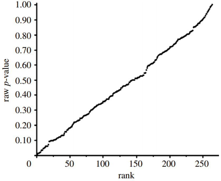
P-value plotting likewise reveals randomness, no significant association, when applied in Figure 4 to a meta-analysis that combined data from 69 questions drawn from 40 observational studies. The claim being evaluated in the meta-analysis was whether long-term exercise training of elderly is positively associated with greater mortality and morbidity (increased accidents and falls and hospitalization due to accidents and falls).

Figure 4: P-value Plot, 69 Questions Drawn From 40 Observational Studies, Meta-analysis of Observational Data Sets Analyzing Association Between Elderly Long-term Exercise Training and Mortality and Morbidity Risk⁹⁷

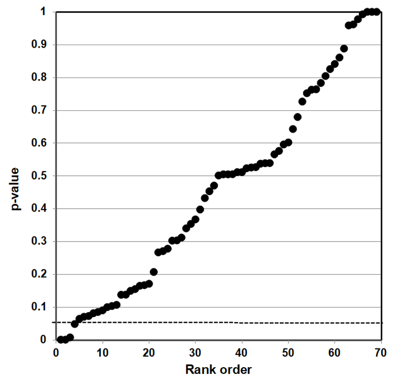
Figure 4, as Figure 3, plots the p-values as a sloped line from left to right at approximately 45-degrees, and therefore supports the presumption of randomness. Note that Figure 4 contains four p-values less than 0.05, as well as several p-values close to 1.000. The p-values below p = 0.05 are most likely false positives.

These claims are purely statistical. Researchers can, and will, argue that discipline-specific information justifies treating their particular claim for a statistical association—that “relevant biological knowledge,” for example, supports the claim that there truly is an association between breakfast cereal consumption and boy-baby conception.⁹⁸

We recognize the possibility where statisticians and disciplinary specialists talk past one another and refuse to engage with the substance of one another’s arguments. But we urge disciplinary specialists, and the public at large, to consider how extraordinarily unlikely it is for a p-value plot indicating randomness to itself be a false positive. The counter-argument that a particular result truly registers a significant association needs to refute the chances against such a 45 degree line appearing if the individual results were not the consequence of selecting false positives for publication.

Such a counter-argument should also consider that p-value plotting does register true effects. We applied the same method to produce a p-value plot in Figure 5 of studies that examined a smoking-lung cancer association.

Figure 5: P-value Plot, 102 Studies, Association of Smoking and Squamous Cell Carcinoma of the Lungs⁹⁹

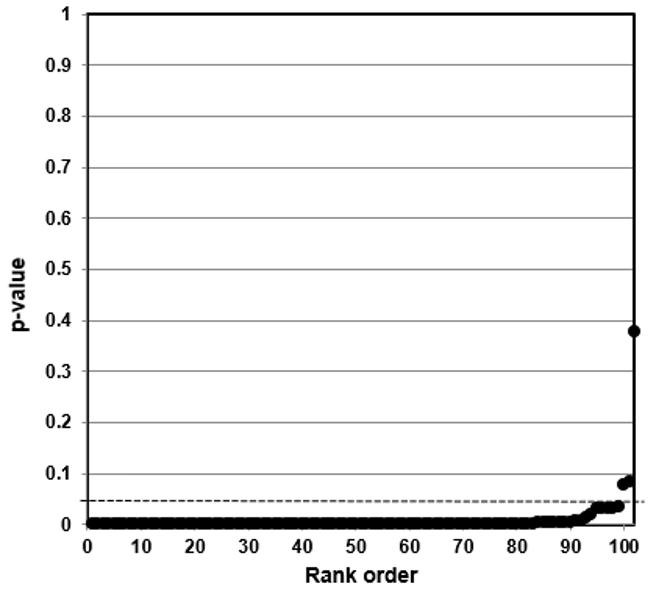
In this case, the p-value plot did not form a roughly 45-degree line, with uniform p-value distribution over the interval. Instead it formed an almost horizontal line, with the vast majority of the results well below p = 0.01. Only 3 out of 102 p-values were above p = 0.05. One outlying p-value was just below 0.40—which reminds us that even where there is a true strong relationship, a few studies may produce false negatives. Our p-value plot provides evidence that the studies associating smoking and lung cancer had discovered a true association.

Bilinear P-value Plots

Our method also registers bilinear results (divides into two lines). In Figure 6, we plotted studies that analyze associations between fine particulate matter and the risk of preterm birth or term low birth weight. A 45-degree line as in Figures 3 and 4 indicates randomness, no effect, and therefore strongly suggests that researchers have indulged in HARKing if they claim a positive effect. A bilinear shape instead suggests the possibility of publication bias, p-hacking, and/or HARKing—although there remains some possibility of a true effect.

Figure 6: P-value Plot, 23 Studies, Association of Fine Particulate Matter (PM_2.5) and the Risk of Preterm Birth or Term Low Birth Weight¹⁰⁰

As we shall explain, such a bilinear plot should usually be interpreted as providing evidence that bias described above has affected a given field, albeit not as strong as the evidence that a 45-degree line provides evidence of no effect. Still, researchers would have good cause to query a claim of an association between fine particulate matter and the risk of preterm birth or term low birth weight, even if a true effect cannot be absolutely ruled out.

Figure 5 demonstrates that our method can detect true associations—it will not come back with a 45-degree line no matter what data you feed into it. When it does detect randomness, as in Figure 3 and 4, the inference is that a particular result is likely to be random, and that the claimed result has failed a statistical test that a true positive body of research passes.

When a p-value plot exhibits bilinearity, as in Figure 6, that provides evidence that there are 1) missing p-values—missing results, which ought to complete the (null) line; and/or 2) p-hacked results, which have driven results down from what they should be to results smaller than the professionally designated level of statistical significance. Bilinearity, in other words, provides evidence that a field has been subject to publication bias—either that negative results have gone into the file drawer or that published results are the result of p-hacking, and/or HARKing.

Our test is useful for assessing the scientific literature precisely because it provides reasonable possibilities for both success and failure.¹⁰¹ We should emphasize that this method is not meant to present an unanswerable disproof of any study or literature to which it is applied. As noted above, the authors of the claim associating maternal breakfast cereal consumption with altered fetal sex ratios made a counter-argument to our critique, and to the argument for randomness displayed in Figure 3. We urge all scholars and interested citizens to examine these counter-arguments. Scientific discovery proceeds by the scrutiny of such arguments and counter-arguments.¹⁰²

We claim that our p-value plot method provides a useful test to check claims against the null-hypothesis. Any such claims ought as a general rule to survive the test of our method—particularly if they are to be used to influence government policy.

P-value plots are an essential component of the rigorous statistical testing that must now be considered the scientific gold standard. Even meta-analyses exclusively relying on studies of RCTs, which use admirably rigorous study designs,¹⁰³ can display bilinear p-value plots. P-value plotting provides evidence that while RCT studies may be necessary to produce rigorous science, they are not sufficient unless they have been subjected to equally rigorous statistical testing. (For three additional examples of p-value plots that register bilinear results, see Appendix 3: Common Examples of Bilinear P-value Plot Behavior.)

Meta-Analyses: Definition and Use

Now that we have explained how p-value plotting works, we define what a meta-analysis is and how they are used together to evaluate the reliability of a claim. A meta-analysis is a systematic procedure for statistically combining data from multiple published papers that address a common research question—for example, whether a specific factor is a likely cause or origin of a health outcome such as a stroke or a heart attack. Scientists can conduct meta-analyses relatively easily. Researchers use computer programs to search the published literature, sort quickly through titles, abstracts, and full-texts of papers, and select ca. 10−20 papers from the hundreds to thousands of papers initially identified as candidates for meta-analysis.

The set of papers chosen for a single meta-analysis itself requires careful study so as to select properly comparable and on-topic papers and include all the relevant studies.¹⁰⁴ In the well-established cottage industry of meta-analysis studies, a skilled team of 5−15 researchers can turn out one meta-analysis per week.¹⁰⁵ Researchers publish approximately 5,000 meta-analysis studies per year.¹⁰⁶

Many government agencies now depend upon meta-analyses. The flood of papers on any given topic makes it difficult even for an expert to stay abreast of all the literature, and a meta-analysis provides a convenient way to digest the results of many individual papers. Government agencies also wish to base their policy on a broad spectrum of rigorous, comparable research, rather than just one or a few individual studies. Meta-analyses offer the promise that government agencies are indeed using such research. Meta-analyses also offer what appears to be an impartial protocol that can provide a safeguard against the danger of biased expert judgment.

Yet meta-analyses have not proved to be a cure-all. Meta-analyses can themselves be affected by publication bias, and almost every other form of irreproducibility-crisis research error that affects individual studies.¹⁰⁷ For example, when researchers vary meta-analyses’ inclusion and exclusion criteria—the criteria stating which studies to include in a meta-analysis and which to exclude—they can produce wildly varying results.¹⁰⁸ In other words, researchers who do not pre-register their inclusion and exclusion criteria can HARK their meta-analyses.

Meta-analyses’ reliability also depends on their base studies’ reliability—and if those have been affected by publication bias or other infirmities (e.g., failure to apply MTMM to control for experiment-wise error), then the meta-analyses they are conducting are no more than Garbage In, Garbage Out (GIGO). Funding bias can affect meta-analyses—and where government agencies are concerned, it is worth emphasizing that government funding can produce substantial funding bias.¹⁰⁹

Meta-Analyses: Evaluation

Qualitative study of meta-analyses is a burgeoning field, which should repay further development.¹¹⁰ We will focus here, however, on the quantitative, statistical study of meta-analyses’ validity—an approach made possible by the extraordinary growth in the number of meta-analyses.

When we refer to a research ‘claim’ in our discussion below, we mean that a study makes a claim of a positive association between a factor investigated and an outcome based on finding small p-values (less than 0.05) in their research. As it is a statistical claim being made by the meta-analysis researchers, we can evaluate the reliability of the claim from a statistical point-of-view. We can use p-value plotting to evaluate published meta-analyses, as we did in Figures 3—6, and thereby uncover problems in the way these meta-analyses have been interpreted.

When we plot an approximately 45-degree line, we acquire good evidence for the null hypothesis. When we plot bilinearity, we acquire evidence of publication bias, p-hacking, and/or HARKing—and significant evidence against any claim of a consistent overall positive association between cause and outcome across the studies used in that particular meta-analysis. At the very least, we have acquired evidence that some unidentified covariate complicates the putative relationship.¹¹¹

We noted above that government agencies rely heavily on meta-analyses to justify regulation. They do not as yet subject these meta-analyses to p-value plotting—and we believe that their failure to do so denies them a very useful tool for assessing the validity of such meta-analyses. P-value plotting that establishes bilinearity does not disprove the meta-analysis. The significant associations could be true; the random results in error. But given the known incentives toward publication bias, p-hacking, and HARKing, bilinearity says we should take meta-analyses’ claims to have detected positive associations with a big grain of salt.

Where government regulatory policy depends on the claim that such positive associations exist, the existence of a bilinear p-value plot provides a very strong argument that a body of literature has not actually proved the existence of an association to the level that justifies government regulation. A bilinear p-value plot provides a good rule of thumb: a government agency has not yet acquired the rigorously tested body of scientific research needed to justify regulation.

P-value plotting isn’t itself a cure-all. The procedure might not be able to tell when an entire literature consists of biased results. P-value plotting cannot detect every form of systematic error. But it is a useful tool, which allows us to detect a strong likelihood that a substantial portion of government regulation has been built on inconsistent science.

We note here that p-value plotting is not the only means available by which to detect publication bias, p-hacking, and HARKing in meta-analyses. Scientists have come up with a broad variety of statistical tests to account for such frailties in base studies as they compute meta-analyses. Unfortunately, publication bias and questionable research procedures in base studies severely degrade the utility of existing means of detection.¹¹² We proffer p-value plotting not as the first means to detect publication bias and p-hacking in meta-analyses, but as a better means than alternatives which have proven ineffective.

The EPA and PM_2.5

A general concern with air quality in America emerged in the late 1940s and early 1950s, precipitated by chronic smog in Los Angeles, the freak but deadly combination of weather and airborne emissions in 1948 at Donora, Pennsylvania, and London’s Great Smog of 1952. These three incidents, and the newly revived recollection of a similarly deadly freak combination of weather and airborne emissions in 1930 in the Meuse Valley in Belgium, sparked increasing concern with a range of airborne components, such as oxides of sulfur, nitric and nitrous oxides (i.e., NO and NO₂), and particulate matter—independent of whether they contributed to visually perceptible smoke. Smog became a household world. The federal government’s Public Health Service turned its attention to the general effects of airborne components on health.¹¹³

A series of local and state regulatory initiatives, particularly in Los Angeles and California, led to the establishment of a federal regulatory structure in 1963—The Clean Air Act. This was followed by further federal measures, notably the Motor Vehicle Control Act (1965), the Clean Air Act Amendments (1966), the Air Quality Act (1967), the Clean Air Act Amendments (1970), and the establishment of the Environmental Protection Agency (1970). These collectively, but particularly the last two, set the ground rules for the regulatory structure that has persisted to the present day.¹¹⁴

The EPA must develop air quality criteria for specific airborne components, informed by expert opinion, and describe their effects singly and in combination on the health and welfare of American citizens. The EPA must set National Ambient Air Quality Standards (NAAQS), as a yardstick by which states and localities can measure their own air quality, and as a legal requirement to enforce reduction of airborne components.

These NAAQS are for carbon monoxide (CO), hydrocarbons (HC), lead (Pb), nitric oxides (NO_x), ozone (O₃₎, particulate matter (PM), and oxides of sulfur (SO_x). It must also review the NAAQS periodically, to determine whether further regulation is in order. The EPA acts in coordination with different federal government departments, such as the Office of Management and Budget (OMB) and the Council on Environmental Quality (CEQ), but it plays the leading role.¹¹⁵

Costs
The costs of insufficiently substantiated regulation can become exorbitant. As a recent example, consider estimated costs requiring ships to use “cleaner fuel” with less sulfur, so as to reduce SO₂ emissions.¹¹⁶ The EPA argues that the move to low-sulfur ship fuel could save up to 14,000 American and Canadian lives every year. The inferred health-related benefits are estimated to be as much as US$110 billion/year in 2020. The EU claims these regulations will prevent 50,000 premature deaths. On the other hand, the cost of these regulations is estimated at US$3.2 billion/year in 2020 and may rise to a total of one trillion dollars through the year 2050.¹¹⁷

Yet a growing body of research fails to support the EPA and the EU’s mortality claims.¹¹⁸ This research provides evidence that SO₂ in ambient air has no significant association with mortality,¹¹⁹ heart attacks,¹²⁰ asthma,¹²¹ or lung cancer.¹²² We may be paying up to $1 trillion dollars to satisfy a regulation with no real scientific foundation.

The EPA issues an extraordinary number of regulations, which affect every area of the economy and constrict everyday freedoms. If the long-term cost of one regulation on one industry amounts to one trillion dollars, the cost of many regulations on every industry is uncountable trillions. The EPA should only impose such costly regulations using fully reproducible science that has survived a battery of severe tests.

The EPA slowly imposed increasingly restrictive regulations and regularly updated NAAQS (Figure 7). These required the accumulation of data on both air quality and on health effects—even forwarded by the EPA’s sponsorship of research that would underpin the emerging regulations. The EPA only shifted from regulation of Total Suspended Particles (TSP) to PM₁₀ in 1987. It did not regulate PM_2.5 explicitly until 1997. The EPA is far older than its current regulatory regime for particulate matter.¹²³

Figure 7: Summary of particulate matter (PM) National Ambient Air Quality Standards (NAAQS) implemented by the U.S. Environmental Protection Agency (U.S. EPA)¹²⁴

Year Implemented	Indicator	24 hr Average (µg/m^3)	Statistical Form for 24 hr Average	Annual Average (µg/m^3)	Statistical Form for Annual Average
1971	TSP	260	Not to be exceeded more than once per year	75	Annual geometric mean
1987	PM10	150	Not to be exceeded more than once per year on average over a three-year period	50	Annual arithmetic mean averaged over three years
1997	PM2.5	65	98th percentile averaged over three years	15	Annual arithmetic mean averaged over three years
2006	PM10	150	Same as 1987 NAAQS	None	Annual average was vacated
2006	PM2.5	35	98th percentile averaged over three years	15	Same as 1997 NAAQS
2013	PM10	150	Same as 1987 NAAQS	None	Annual average was vacated in 2006
2013	PM2.5	35	Same as 2006 NAAQS	12	Annual arithmetic mean averaged over three years

The current regulations depend on statistical analysis. The EPA and environmental epidemiologists, as a discipline, have not established direct causal biological mechanisms that link air components and health outcomes¹²⁵ —save for freak conditions such as prevailed in the Meuse Valley (1930), Donora (1948), and London (1952).¹²⁶

Rather, they have relied on statistical analyses to discern significant associations between air components and health outcomes. These associations provide the “proof” that an air component, alone or in association with other elements, causes damage to health and to the economy. The debate about whether or not the EPA should make a particular regulatory decision raises questions central to the irreproducibility crisis—data accuracy, research protocols, statistical analyses, publication bias, sponsorship bias, etc.

We note here a conundrum. By an extraordinary number of indicators, Americans’ general health has risen remarkably over the last several generations.¹²⁷ The gravest recent harm to Americans’ life expectancy has been the opioid epidemic, concentrated among poor white Americans—an effect entirely unrelated to the remit of the EPA.¹²⁸ Yet the EPA produces an ever-lengthening catalogue of studies of things that harm Americans’ health.¹²⁹ Feinstein charged as far back as 1988 that much of the research suggesting specific health-harms must be the result of misuse of statistics and computers, data dredging to produce dire literature of statistically significant effects that square badly with evidence of general improvements in health and life expectancy.¹³⁰

Who Benefits?
The EPA appears to have acted selectively in its approach to the health effects of PM_2.5. In the early 1990s two different set of researchers examined the health effects of PM_2.5 and mortality. Dockery et al. published a study that appeared in the New England Journal of Medicine in 1993 that found a significant association between small particulate matter in outdoor air and death rates; the Dockery study received apparent support from the study by his colleagues in Pope et al. in 1995.¹³¹ Yet Styer et al. published a study in 1995 that drew upon a far larger data set and found no association between particulate matter in outdoor air and deaths.¹³²

The EPA had funded both Dockery and Styer—but at that point, the EPA ceased funding the Styer group and began intensive support of the Dockery-Pope line of research, despite substantial skepticism from the scientific community about the accuracy of the Dockery-Pope data.¹³³ The Health Effects Institute (HEI), half-funded by the EPA, then re-analyzed the data and supported the claims made in the Dockery and Pope studies—but without ever making their data set available to the public or to the EPA.¹³⁴ HEI neither requested nor examined the Styer data set.¹³⁵

The EPA has continued to pay more attention to research that supports regulation. In 2009, the EPA’s Integrated Science Assessment for Particulate Matter repeatedly cited meta-analyses that supported EPA regulatory policy, while failing to cite key negative papers in the literature or citing perfunctorily by way of brusque and insufficiently justified dismissal.¹³⁶

More narrowly, the EPA constructed its PM_2.5 regulation from 1997 to the present day upon a series of studies in the generation from the 1970s to the 1990s that sought to establish: 1) significant associations between PM_2.5 and various health effects; and 2) that the health effects were themselves substantial enough to justify EPA regulation.¹³⁷ The regulation from 1997 onward relies on research drawn from the famous Harvard Six Cities and American Cancer Society (ACS) studies—whose original data, on claimed grounds of privacy and confidentiality, have never been made transparently available to other researchers for reproduction or critique.¹³⁸

We may note here that data for environmental epidemiology is difficult to collect—it is an observational science rather than a laboratory one, and one that requires data sets of hundreds of thousands of individuals, sometimes collected over decades, to make any sort of definitive statement. The EPA delayed more rigorous regulation of PM_2.5 for a generation precisely so as to assemble a data set that they thought would justify such regulation. The EPA and its advocates argue that the difficulty of collecting such data justifies allowing the EPA to base regulation on inaccessible data.

However, it is precisely because the data are so difficult to collect that it is vital to have access to the one available data set, so that it may be subjected to a battery of rigorous (severe) tests to see if the analysis is sound. The burden of proof for transparency and reproducibility lies with the research the EPA uses as the basis for its regulations.

When EPA regulation is based on inaccessible data, there are numerous potential weaknesses. We cannot fully account for interaction effects—the effects of “confounding” variables on health effects, such as temperature,¹³⁹ atmospheric inversion, or varying demographic predispositions to sickness and mortality.¹⁴⁰ We cannot examine the base information itself for reliability. Death certificates, for example, are not entirely reliable sources of information.¹⁴¹

Neither do we possess the data that can begin to allow us to determine what are the precise causal mechanisms—the biological mechanisms—by which an airborne component actually induces a health risk.¹⁴² (For more discussion about current status of unanswered PM_2.5-mortality causal mechanisms and several negative studies that invalidate PM_2.5-mortality causation, see Appendix 4: PM2.5−Mortality Causality—Incomplete Evidence. This evidence, drawn from published literature, does not support a PM_2.5-mortality causal mechanism.)

The Harvard Six Cities/ACS data that underpin the Dockery/Pope research has never been subjected to Multiple Testing and Multiple Modeling (MTMM), even though an adjustment for MTMM with the widely-used SAS statistical software could easily be applied to the data.¹⁴³ Since Dockery and Pope never made the data publicly available, no independent, critical researcher can subject the Harvard Six Cities/ACS data to the severe test of MTMM. Since analysis of newer and much larger data sets has found no effects of air quality on mortality, skepticism about the Dockery/Pope results is warranted.¹⁴⁴

We would prefer to analyze the EPA’s PM_2.5 policy by subjecting the data underlying the Harvard Six Cities/ACS studies to further scrutiny. Unfortunately, such scrutiny is impossible because the data’s owners have barred public access on the claimed grounds of privacy and confidentiality. Yet p-value plotting provides a way to apply a severe test to results where the data remain hidden, and to assess whether publication bias, p-hacking, or HARKing has produced the body of literature that “justified” the EPA’s PM_2.5 regulation.

Evaluation of PM_2.5 Research Underlying EPA Regulation

Introduction

Environmental epidemiological researchers regularly engage in massive hypothesis tests without making Multiple Testing and Multiple Modeling (MTMM) statistical corrections. These tests have associated air quality components with a remarkable number of possible adverse health effects.

These effects include but are not limited to: all-cause mortality; cause-specific mortality; all-cause morbidity; low birth weight; miscarriage; COPD exacerbation; inflammation; pulmonary complication; autism; obesity; depression; atopic dermatitis; impaired vestibular function (sense of balance); metabolic disorders; suicide, mental health and well-being; ADHD (Attention Deficit/Hyperactivity Disorder); respiratory complication; pneumonia and acute respiratory infection; reproductive outcomes; high blood pressure; lung and other cancers; and accelerated brain aging.¹⁴⁵

Below we summarize four technical investigations about associations between fine particulate matter (PM_2.5) (and in some cases other air quality components) in ambient air with various health effects. These effects include all-cause mortality, heart attacks and two asthma effects—development of asthma and asthma attacks. The investigation on heart attacks using p-value plots has already been published.¹⁴⁶ Preprints of the two forthcoming investigations on asthma have been deposited in the open-access repository arXiv,¹⁴⁷ as has the preprint of a shorter investigation on all-cause mortality.¹⁴⁸

These investigations, whose research protocol we pre-registered,¹⁴⁹ have been or will be submitted to professional journals for peer review and publication. Data used in these studies are publicly available. We approached these investigations by focusing on meta-analyses that ask the specific question whether inferred exposure to PM_2.5 (and other air quality components) is associated with increases in all-cause mortality, heart attacks and asthma. We present strong statistical evidence that the EPA has developed policy and regulated PM_2.5 based upon a field of epidemiology research substantially affected by some combination of sampling bias, publication bias, and/or p-hacking.

Our research also demonstrates more generally how p-value plots may be used to evaluate the reliability of studies making research claims about any air quality component−health outcome associations. Here we present counts and p-value plots for these investigations and then we interpret and discuss them. (For supporting information for these investigations, see Appendix 5: Supporting Information for Investigations of PM2.5-Health Effect Association. This information includes explaining how these counts were made.)

P-Value Plots

All-cause Mortality

The very multiplicity of claimed associations between air components and adverse health effects¹⁵⁰ suggests that even larger numbers of possible hypothesis tests lie behind claims of air quality component associations with all-cause mortality. Claims associating air quality components with all-cause mortality require more than usual care when making MTMM corrections.

The standard six air quality components that environmental epidemiology researchers investigate for associations with all-cause mortality are CO (carbon monoxide), NO₂ (nitrogen dioxide), O₃ (ozone), PM_2.5 (particulate matter, small), PM₁₀ (particulate matter, not as small) and SO₂ (sulfur dioxide). Our investigation of the reliability of data from studies used in a meta-analysis of short-term air quality−all-cause mortality associations focused on NO₂, O₃, PM_2.5, and PM₁₀as “causes”, and all-cause and cause-specific mortalities as “outcomes.”¹⁵¹

In this large-scale systematic review and meta-analysis, researchers reviewed 1,632 papers and selected 196 for analysis. The researchers claimed that, “This study found evidence of a positive association between short-term exposure to PM₁₀, PM_2.5, NO₂, and O₃ and all-cause mortality, and between PM₁₀ and PM_2.5 and cardiovascular, respiratory and cerebrovascular mortality.” The researchers provided risk ratios with confidence limits and from these we produced a p-value plot (Figure 8).

Figure 8: P-value plot, All-Cause Mortality and PM_2.5¹⁵²

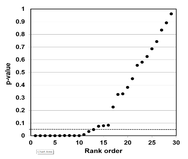
Heart Attacks

Much environmental epidemiology literature claims that poor air quality can trigger a heart attack.¹⁵³ The standard six air quality components that environmental epidemiology researchers identify as heart attack triggers are CO, NO₂, O₃, PM_2.5, PM₁₀ and SO₂. We recently published an investigation of the reliability of data from studies used in a meta-analysis of short-term air quality−heart attack associations.¹⁵⁴

The meta-analysis, which identified and drew data from 34 studies that statistically examined associations between the air quality components and heart attacks,¹⁵⁵ claimed that, “All the main air pollutants, with the exception of ozone, were significantly associated with a near-term increase in MI [myocardial infarction, aka heart attack] risk.”

We counted the number of outcomes, predictors, covariates and time lags¹⁵⁶ used in each of the 34 studies in order to estimate the number of statistical tests performed. Summary statistics for these counts are shown in Figure 9. We also developed p-value plots for the six air quality components (shown in Figure 10).

Figure 9: Summary statistics, Analysis search space (number of statistical tests), 34 studies, associations between air quality components and heart attacks

Statistic	Space1	Space2	Space3
minimum	8	8	240
lower quartile	23	64	2,496
median	36	256	12,288
upper quartile	109	1,024	58,368
maximum	540	16,384	4,587,520

In Figure 9, Minimum = minimum count; lower quartile = 25th percentile count; median = 50th percentile count; upper quartile = 75th percentile count; maximum = maximum count; Space 1 = Outcomes x Predictors x Lags; Space 2 = 2^Covariates; Space 3 (analysis search space or number of statistical tests) = Space 1 x Space 2.

Figure 10: P-value plots, Six air quality components, Air quality−heart attack meta-analysis

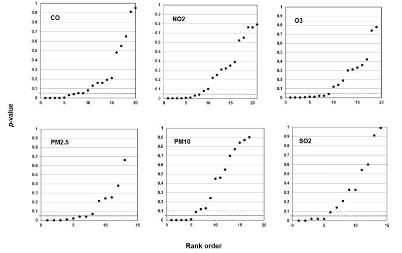
Development of Asthma (Cohort Studies)

We investigated a meta-analysis examining the association of ambient exposure to NO₂ and PM_2.5 early in life with development of asthma later in life.¹⁵⁷ The meta-analysis drew data from 19 published studies involving 18 different cohort populations—13 cohorts for NO₂ and 5 cohorts for PM_2.5. The meta-analysis claimed that, “The results are consistent with an effect of outdoor air pollution on asthma incidence.”

We counted the number of outcomes, predictors and covariates available in each of the 19 studies in order to estimate the number of statistical tests performed. Summary statistics for these counts are shown in Figure 11. We developed a combined p-value plot for NO₂ and PM_2.5 (Figure 12).

Figure 11: Summary statistics, Analysis search space (number of statistical tests), 19 studies, associations between NO₂, PM_2.5 and development of asthma

Statistic	Space1	Space2	Space3
minimum	2	32	96
lower quartile	15	96	1,536
median	24	256	13,824
upper quartile	84	3,072	221,184
maximum	160	262,144	42,000,000

In Figure 11, Minimum = minimum count; lower quartile = 25th percentile count; median = 50th percentile count; upper quartile = 75th percentile count; maximum = maximum count; Space 1 = Outcomes x Predictors; Space 2 = 2^Covariates; Space 3 (analysis search space or number of statistical tests) = Space 1 x Space 2.

Figure 12: 18 Cohort Studies, P-Value Plot¹⁵⁸

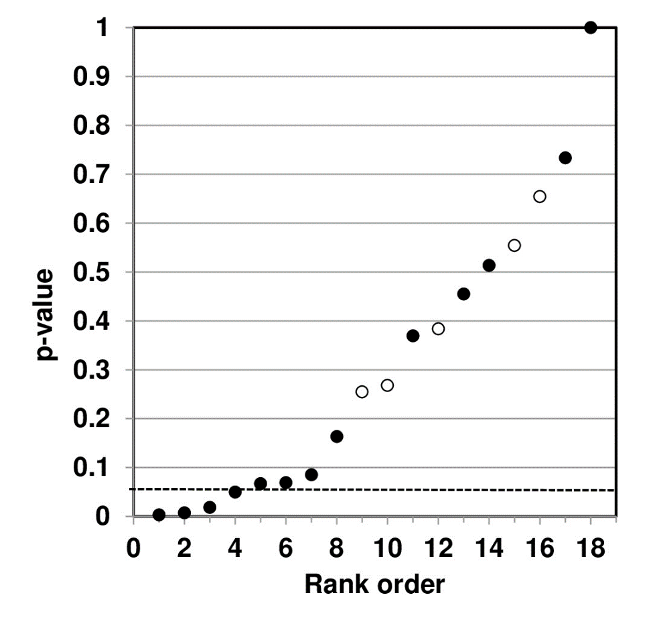
Note: solid circles (●) are NO₂ p-values; open circles (o) are PM_2.5 p-values).

Asthma Attacks (Time-Series Studies)

Much environmental epidemiology literature claims that poor air quality can trigger asthma attacks.¹⁵⁹ We investigated a meta-analysis examining the association of short-term ambient exposure to six air components (CO, NO₂, O₃, PM_2.5, PM₁₀, and SO₂) with asthma attacks.

The meta-analysis drew data from 87 time-series studies that statistically examined associations among air quality components and asthma attacks¹⁶⁰ and claimed that “Short-term exposures to air pollutants account for increased risks of asthma [attack]-related emergency room visits and hospitalizations that constitute a considerable healthcare utilization and socioeconomic burden.”

We counted the number of outcomes, predictors, covariates and time lags available in 17 studies randomly selected from the list of 87 (or 20%) in order to estimate the number of statistical tests performed. Summary statistics for these counts are shown in Figure 13. We made p-value plots for the six air quality components (Figure 14).

Figure 13: Summary statistics, Analysis search space (number of statistical tests), 17 randomly selected studies, associations between air quality components and asthma attack

Statistic	Space1	Space2	Space3
minimum	6	4	96
lower quartile	60	16	1,536
median	160	32	15,360
upper quartile	288	256	40,960
maximum	5,120	512	89,600

In Figure 13, Minimum = minimum count; lower quartile = 25th percentile count; median = 50th percentile count; upper quartile = 75th percentile count; maximum = maximum count; Space 1 = Outcomes x Predictors x Lags; Space 2 = 2^Covariates; Space 3 (analysis search space or number of statistical tests) = Space 1 x Space 2.

Figure 14: P-value plots, Six air quality components, Air quality−asthma attack meta-analysis

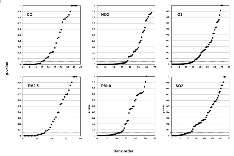
Discussion

Counts

We provided search space counts as estimates of the number of statistical tests performed in base studies for the three air component−health effect meta-analyses we investigated. These include: Figure 9 (heart attack), Figure 11(development of asthma) and Figure 13 (asthma attack). There is known flexibility available to researchers to undertake a range of statistical tests and use different statistical models during observational studies, and then to select, use, and report only a portion of the test and model results.¹⁶¹ Wicherts refers to this flexibility as “researcher degrees of freedom” in the psychological sciences.¹⁶²

Base papers with large search space counts suggest the use of large numbers of statistical tests and statistical models and the potential for researchers to search through and report only a portion of their results (i.e., positive, statistically significant results). In looking at the Space 3 counts in Figures 9, 11, and 13, large numbers of statistical tests performed are a common feature of base studies used in these meta-analyses. For example, estimates of the median number of statistical tests performed in the meta-analyses base papers are 12,288 (34 base papers for heart attack), 13,824 (19 base papers for development of asthma) and 15,360 (17 base papers for asthma attack).

Overall, these three meta-analysis investigations involved estimating search space counts from 70 environmental epidemiology base papers investigating associations between air quality components and health effects. The estimated median number of statistical tests performed for these 70 base papers is 13,056. Given a study with 13,056 statistical tests, we may expect see as many as 0.05 x 13,056 = 653 results with p-values less than 0.05 due to chance alone. Another noteworthy feature of these base studies is that large numbers of statistical test results may have gone unreported in these studies—presumably, results with p-values greater than 0.05.

P-value Plots

We restate how the p-value plots were interpreted:

• A p-value plot that forms approximately a 45-degree line provides evidence of randomness—supporting the null hypothesis of no significant association.
• A p-value plot that forms approximately a line with slope < 1, where most of the p-values are small (less than 0.05), provides evidence for a real effect—supporting a statistically significant association.
• A p-value plot that exhibits bilinearity—that divides into two lines—provides evidence of publication bias, p-hacking, and/or HARKing.¹⁶³

When we examine the specific p-value plots that we created (Figures 8, 10, 12, and 14), the patterns strikingly resemble the bilinear patterns depicted in Figure 6 and the figures shown in Appendix 3: Common Examples of Bilinear P-value Plot Behavior. The bilinear patterns register heterogeneous sets of p-values—two-component mixtures.

These plots imply a mixture of random results and results plausibly due to publication bias, p-hacking, and/or HARKing. There is no consistent effect across studies that we would expect if the data supported a true positive association that represents an alternative hypothesis outcome (i.e., Figure 5).

For example, the PM_2.5 all-cause mortality bilinear p-value plot (Figure 8) presents 29 p-values—13 of these p-values are less than 0.05 and 16 are greater. The meta-analysis’ claim that “this study found evidence of a positive association between short-term exposure to PM_2.5 and all-cause mortality” is not supported by convincing evidence. This result warrants further scrutiny of the researchers’ other claims. For example, p-value plots for PM₁₀, NO₂ and O₃, not shown here, are also bilinear.

The six air component−heart attack p-value plots shown in Figure 10 resemble bilinear patterns. Likewise, bilinearity is a feature of the PM_2.5, NO₂−asthma development p-value plot (Figure 12) and the six air component−asthma attack p-value plots (Figure 14). Bilinear patterns argue that any claim for a general implication of an air components as a cause of heart attack, development of asthma, or asthma attack is without statistical support. We believe that these investigations strengthen our larger argument that all such claims of associations warrant more skepticism than they have so far received.

Findings

We do not claim that our results absolutely disprove claims there are associations between PM_2.5 and all-cause mortality, heart attacks, or asthma complications. Yet they are certainly consistent with the general claim that false-positive results from publication bias, p-hacking, and/or HARKing are common features of the biomedical literature today, including the broad range of risk factor−chronic disease research.¹⁶⁴

Given the large numbers of statistical tests available in the environmental epidemiology base studies used for three meta-analyses we investigated (Figures 9, 11, 13), p-hacking certainly cannot be ruled out as an explanation for the small p-values, less than 0.05, shown in Figures 10, 12 and 14.

We do claim that air component−health effect associations ought to survive a battery of severe but passable tests, such as p-value plots that we have undertaken here. This battery of tests should also include a resampling-based multiplicity analysis (multiple testing and multiple analysis) of the base studies used in a meta-analysis.

Researchers always have the burden of proof to provide a significant association—and government regulators have the higher barrier to prove that an entire body of the best available science supports the requirement to substitute regulation for liberty. It should disturb scientists, bureaucrats, politicians, and citizens alike that current governmental procedures to test for the best available science have failed to pass our test—which is simple to execute, and now widely used in a variety of scientific disciplines.¹⁶⁵

The EPA might not have regulated PM_2.5 at all if they had applied more rigorous scientific reproducibility requirements to research that they used to justify their regulations. Certainly, the EPA policy and regulatory process would have followed a substantially different course. If the EPA were to apply more rigorous scientific reproducibility standards going forward— including p-value plotting in their regular assessments of scientific research—it would vastly improve the scientific reliability of future PM_2.5 regulation.

Conclusion

Overview

Many people ask, what proof is there that the irreproducibility crisis has actually affected existing government regulations? Our p-value plots provide a direct answer to that question. Wherever we apply our p-value plots to a meta-analysis and produce a bilinear relationship, we should presume that the questionable research procedures, HARKing, and p-hacking that constitute the irreproducibility crisis have rendered the underlying research untrustworthy. We have applied our p-value plots to research that provides the justification for EPA regulation of PM_2.5, and bilinear lines appeared. These bilinear relationships provide strong evidence that the government has based its regulations on unreliable research affected by the irreproducibility crisis.

EPA regulations rely on environmental epidemiological literature, without applying rigorous tests for reproducibility—and without considering the environmental epidemiology discipline’s general refusal to take account of the need for Multiple Testing and Multiple Modeling. Such rigorous tests are needed not least because earlier generations of environmental epidemiologists have already identified the low-hanging fruit.

These include massive statistical correlations between risk factors and health outcomes—e.g., the connection between smoking and lung cancer. Modern environmental epidemiologists habitually seek out small but (nominally) significant risk factors and health outcome associations. These practices render their research susceptible to registering false positives as real results, and to risk mistaking an improperly controlled covariable for a positive association.

Environmental epidemiologists are aware of these difficulties, but, despite having remade their discipline into an exercise in applied statistics, they do little to control for bias, p-hacking, and other well-known statistical errors.¹⁶⁶ The intellectual leaders of their discipline have positively counseled against taking measures to avoid these pitfalls.¹⁶⁷

But environmental epidemiologists, and the bureaucrats who depend on their work to support regulations, proceed as a field with self-confidence, and an insufficient sense of the need for a humble awareness of just how much statistics must remain an exercise in measuring uncertainty rather than establishing certainty.¹⁶⁸ Their results do not possess an adequate scientific foundation. Their so-called “facts” are built on shifting sands, not on the solid rock of real, transparent, and critically reviewed scientific inquiry.

Our study shows how one particular set of statistical techniques, simple counting and p-value plots, can provide a severe test of environmental epidemiology meta-analyses to detect p-hacking and other frailties in the underlying scholarly literature. We have used these techniques to demonstrate that meta-analyses associating PM_2.5 and other air quality components with mortality, heart attacks and asthma attacks fail this severe test.

Our study also demonstrates negligence on the part of both environmental epidemiologists and the EPA. The discipline of environmental epidemiology has failed to adopt a simple statistical procedure to test their research. The EPA has failed to require that research justifying regulation be subjected to such a test. These persistent failures undercut confidence in their professional capacities, as researchers and as regulators.

These failures also suggest that, more broadly, the standard procedures of environmental epidemiology are insufficiently rigorous. These failures also suggest that current EPA regulatory policy, both in general and with regards to PM_2.5 regulation in particular, fails to test with sufficient rigor the research used to justify regulation. The EPA also makes comprehensive tests impossible by failing to require public access to data sets used to justify regulation. The EPA’s failure to use this particular testing procedure is symptomatic of a larger failure to incorporate a full range of severe statistical tests—without which the results of a statistically-founded discipline such as environmental epidemiology cannot qualify as the best available science.

Both environmental epidemiology as a discipline (including foundations, journals, and tenure committees) and the EPA ought to adopt a range of reforms to improve the reproducibility of their research. However, we direct our recommendations to the EPA, and more broadly to federal regulatory and granting agencies.

We have reluctantly come to the conclusion that scientists will not change their practices unless the federal government credibly warns them that it will withhold government grant dollars until they adopt stringent reproducibility reforms. We have also come to the conclusion that federal regulators will not adopt stringent new tests of science underlying regulation unless they are explicitly required to do so.

Yet while these recommendations are framed as suggestions for government requirements, we still urge scientists to adopt these reforms voluntarily.

Recommendations to the EPA

All these recommendations are intended to bring EPA methodologies up to the level of best available science, as per the mandate of The Information Quality Act.¹⁶⁹

1. The EPA should adopt resampling methods (Multiple Testing and Multiple Modeling) as part of its standard battery of tests applied to environmental epidemiology research.

We have critiqued at length the standard procedure of environmental epidemiology meta-analysis, which has proven susceptible to statistical frailties. The corollary of this critique is that the EPA should adopt the standard procedure, elaborated in a work partly written by one of our co-authors more than a quarter century ago,¹⁷⁰ to control for environmental epidemiology’s Multiple Testing and Multiple Modeling (MTMM) problem.

This resampling-based multiple testing procedure already has been incorporated into a variety of disciplines, including genomics¹⁷¹ and economics,¹⁷² and has been shown to be optimal for a broad class of testing problems.¹⁷³ Any discipline using statistics can incorporate these procedures into their regular tests. Any government agency that relies on scientific research can require the use of such procedures to test scientific research, before it is used to justify regulation, or qualify as best available science. The EPA should do so.

The EPA, in other words, should only rely on base studies and meta-analyses that use a resampling methodology (MTMM) to correct their results. The EPA should also subject all such research to independent MTMM analyses.

MTMM analysis is not the only tool that can be used to adjust an analysis for p-hacking and other forms of biased sampling. But we believe it is a useful tool, which can easily be adopted by regulators and researchers to apply a severe test to scientific research. We do not propose it as a cure-all—but as a tool useful in itself, and also as an example: that a variety of reproducibility reforms can practicably be introduced into the ordinary procedures of professional and governmental judgment of scientific validity.

2. The EPA should rely for regulation exclusively on meta-analyses that use tests to take account of endemic questionable research procedures, HARKing, and p-hacking.

Questionable research procedures, HARKing, and p-hacking are endemic in environmental epidemiology—as they are in many disciplines affected by the irreproducibility crisis. Since so many base studies are unreliable, the meta-analyses which collate these base studies likewise have become unreliable—Garbage In, Garbage Out.

When the EPA uses meta-analyses or a systematic review to justify regulation, it should only rely on meta-analyses that conduct rigorous tests to detect whether a field’s base studies have been affected by questionable research procedures, HARKing, and p-hacking. While we will not prescribe further particular methods here, we state that existing tests are not sufficient.¹⁷⁴ The EPA should adopt tests substantially more stringent than those they currently accept.

3. The EPA should redo its assessment of base studies more broadly to take account of endemic questionable research procedures, HARKing, and p-hacking.

The different aspects of the irreproducibility crisis—questionable research procedures, HARKing, and p-hacking—thrive opportunistically within research structures that allow scientists arbitrary control over revealing their questions and their data. When we remove that control, we remove much of the possibility that the irreproducibility crisis will affect government regulation.

The EPA should take the initiative generally to assess base studies with an eye to rooting out questionable research procedures, HARKing, and p-hacking. The EPA can best remove that control by requiring preregistration of research that justifies regulation and public access to research data used to justify regulations.

4. The EPA should require preregistration and registered reports of all research that informs regulation.

Preregistration and registered reports will constrain the ability of scientists to HARK, and generally inhibit p-hacking and questionable research procedures. Preregistration and registered reports are not cures. Determined scientists in time undoubtedly will devise methods to undermine the effectiveness of these precautions. But preregistration and registered reports will substantially improve the reliability of research used by the EPA. The EPA should stipulate that all preregistration and registered reports must detail the MTMM methods that will be used to assess results.

5. The EPA should also require public access to all research data used to justify regulations.

We have provided substantial corroborative evidence that the irreproducibility crisis has affected research used to justify EPA regulation; we cannot provide direct evidence because the EPA does not permit or facilitate public access to that research data. The EPA should require that all research used to justify regulation must provide public access to the underlying research data. The EPA should direct all necessary funding to ensure de-identification of human data.¹⁷⁵ and provide an adequate means to address all privacy and confidentiality concerns. But these are challenges that the EPA can and must meet, not convenient obstacles that prevent public access.¹⁷⁶

6. The EPA should consider the more radical reform of funding data set building and data set analysis separately.

Researchers who combine data collection and data analysis possess a temptation to adjust the data to improve results of their analyses. The EPA should consider separating these two functions, so as to remove the situation that presents this temptation. It should also consider combining this reform with a requirement that researchers provide a hold-out data set to a trusted third party before analysis, so that any analysis claim can be tested independently using the hold-out data set.

7. The EPA should place greater weight on reproduced research.

We have specified the use of improved statistical techniques to reduce the effects of the irreproducibility crisis in environmental epidemiology. But such statistical tests cannot catch every sort of questionable research procedure. Indeed, research that passes every statistical test might still be a false positive. The EPA therefore should increase the weight it assigns to research that is not only reproducible, but also reproduced—and decrease the weight it assigns to research that has not yet been reproduced.

8. The EPA should constrain the use of “weight of evidence” to take account of the irreproducibility crisis.

The “weight of evidence” principle generally facilitates arbitrary judgments as to what science should inform regulation. Self-interest will inevitably incline scientists and regulators, consciously or unconsciously, to weigh more heavily research that facilitates regulation. Groupthink redoubles the effects of consensus-thinking, which too easily discards research that fails to endorse the consensus.

Wherever possible, the EPA should substitute transparent rules for “weight of evidence” judgments. The EPA should also require regulators to elaborate in detail whenever they apply a “weight of evidence” judgment, by means of a coherent argument which can be falsified by independent critique.

9. The EPA should report the proportion of positive results to negative results in the research it funds.

The EPA’s bureaucratic self-interest—and its mandate—will always incline its employees, consciously or unconsciously, to fund research that supports regulation. The EPA must make a conscious effort to ensure that the research it funds does not put a thumb on the scales of the field’s research as a whole—that it does not fund an overabundance of false positive results and then say that the “weight of evidence” justifies regulation.

The EPA should report the proportion of positive to negative results in the research it funds, with data reported for every program and discipline. Here we propose that any program or discipline that reports more than 65% positive results in the research it funds should initiate a reform of its granting program, to counter the effects of bureaucratic self-interest and groupthink.

10. The EPA should not rely on research claims of other organizations until these organizations adopt sound statistical practices. The EPA often funds external organizations, such as the World Health Organization (WHO), the International Agency for Research on Cancer (IARC), and the Health Effects Institute (HEI). These organizations are effectively beyond the reach of effective oversight.

11. The EPA should increase funding to investigate direct causal biological links between substances and health outcomes.

Environmental epidemiology depends on establishing statistical associations in default of establishing direct causal biological links between substances and health outcomes. The EPA’s reliance on association rather than causation weakens the justifications of its regulations. The EPA should redirect grant funding toward investigating direct causal biological links between substances and health outcomes, so as to minimize its reliance on statistical associations. A note of caution, however, is that direct experimentation on humans has been conducted and indications of dire effects have not been found.¹⁷⁷

As a corollary, the EPA also should place substantially greater weight on negative results in research to establish direct causal biological links. They should also establish a set procedure by which a sufficient number of such negative results preclude regulation absent research that proves statistical association to a substantially higher standard of rigor than at present required.

All federal regulatory agencies, wherever relevant, should undertake parallel reforms.

Scope and Implementation

We believe the EPA should not overturn previous regulations arbitrarily as it implements our recommendations.Regulatory stability is an important goal for the Federal government, and indeed for any system of laws and regulations. American enterprises have invested substantial resources in regulatory compliance, and their investments should not casually be set at naught.¹⁷⁸

Extensive regulatory schemes can amount to a competitive advantage to large corporations against small ones, since large companies have the capacity to comply with an extensive regulatory framework. Regulatory stability should not be used to provide an enduring competitive advantage to big business. Furthermore, regulatory costs are borne ultimately by American enterprises’ consumers—American citizens. These costs can have negative health consequences, such as those that follow from increased unemployment.¹⁷⁹

When new data, new analysis, and new theory call into question and overturn previously established science, the regulations that now-discredited science once justified should be dismantled—if not in haste, then with all deliberate speed.¹⁸⁰ These reforms can and should be introduced via the EPA’s regular, planned regulatory reviews—which will allow the reform of procedures to enact new regulations to proceed in an orderly manner.¹⁸¹ But these regulatory reviews should not exempt existing regulations. We should not grandfather bad science forever—or even for very long.

For a highly relevant example, consider the Harvard Six Cities/ACS studies that are cited in support of current PM_2.5 regulation.¹⁸² Enstrom asserts that Pope’s 1995 ACS II paper only achieved statistical significance by “data gardening,” since not all the data that were available were used in the analysis.¹⁸³ Other researchers have also subjected Dockery (1993) to severe criticism.¹⁸⁴ Since the Dockery and Pope studies are not reproducible, and recent negative studies¹⁸⁵ are, then how should the EPA unwind its regulations?

We suggest a multi-part reform. The government should announce that it will cease using the Harvard Six Cities/ACS studies, and similarly irreproducible data sources, by some reasonably near date, unless the underlying data have been made publicly available. As the same time, the government should immediately begin to fund a high-priority program to create a new, substitute data set, with born-open, publicly accessible data and built-in de-identification to address anyprivacy concerns.

These data will then be available for the EPA to use once it ceases using the Harvard Six Cities/ACS studies and similarly irreproducible data sources. If the new data do not justify the regulations, then the regulations can be withdrawn in an orderly manner. If the new data do justify the regulations, then the regulations can be continued. This multi-part reform should maximize reproducibility reforms and regulatory stability.

Similarly crafted multi-part reforms, enacted throughout the EPA’s remit, ought to maximize the twin goods of good science and stable regulation.

Final Considerations

We have used the phrase “irreproducibility crisis” throughout this report—and we should note that distinguished meta-researchers prefer to regard the current state of affairs as an “irreproducibility challenge.”¹⁸⁶ This is a serious caution. While we do think that p-hacking, HARKing, and questionable research procedures are endemic within science, and particularly within environmental epidemiology, we also recognize that not every reader will accept that such a crisis exists.

For such readers, we say that you do not need to believe that there is an irreproducibility crisis. You can believe that it is better to regard these problems as irreproducibility challenges. Whether challenge or crisis, these scientific practices are not the best available science. We should use the best scientific practices simply because they are the best scientific practices. Mediocrity ought not be acceptable.

This applies doubly to the science that underpins government regulation. Statistical research that seeks out associations must justify itself against the null hypothesis. Likewise, regulations that seek to restrict freedom must justify themselves against the null hypothesis of a free republic—that it is better for government to do nothing and for the republic’s citizens to exercise their freedoms untrammeled. Research used to justify government regulations, even more than ordinary research, should survive every rigorous test available before it is taken as credible.

This has long been the spirit of American regulatory policy. Our policymakers, representing the American people, long ago decided that regulations must justify themselves with the best available science—that is, science that has passed the severest tests. They used this phrase to defend liberty, not to facilitate its abrogation; to restrict regulation to the least necessary and not to facilitate the expansion of government regulation. Best available science was meant to restrict government bureaucrats, not to authorize them to build regulatory empires.¹⁸⁷

The reforms we suggest respond partly to the development of a regulatory research regime entirely too fixed on extending regulations, regardless of the underlying science. These reforms also respond to the developing professional and public awareness of the irreproducibility crisis, and its ramifications. Finally, they build on new statistical strategies that have been devised to ensure that we are using the best available science. Even were there no scientific-regulatory complex, even were there no irreproducibility crisis, we would champion government adoption of these new methods to assess research, simply because they are the best methods. The American government should not be constrained by obsolescent methods or secret data as it seeks to judge the best science.

We have subjected the science underpinning PM_2.5 regulation to a serious critique, and we believe the EPA should take account of this critique as it reforms these particular regulations. But we care even more about reforming the procedures the EPA uses in general to assess science—and the procedures used throughout government.

Government regulatory procedure matters far more than any particular implementation of regulatory policy. Validationprocedures for statistical data matter the most of all, regardless of how they affect government policy—for science cannot reliably seek out truth on a foundation of rotten procedure.¹⁸⁸ This report focuses on government regulatory policy, but we must never lose sight of that loftier goal.

The government should use the very best science—whatever the regulatory consequences. Scientists should use the very best research procedures—whatever the result they find. Those principles are the twin keynotes of this report. The very best science and research procedures involve building evidence on the solid rock of transparent, reproducible, and reproduced scientific inquiry; not on shifting sands.

Appendix 1: Multiple Testing and Multiple Modeling (MTMM) and Epidemiology

Multiple Testing and Multiple Modeling (MTMM) controls for experiment-wise error—the probability that at least one individual claim will register a false positive when you conduct multiple statistical tests.¹⁸⁹ It is instructive to trace some of the history with examples of MTMM with respect to epidemiology.

Friedman made a research claim in 1959 that Type A personality was associated with heart attacks.¹⁹⁰ Several later studies failed to replicate these results. Expert committees found fault with these latter studies and the Type Apersonality─heart attack claim lives to this day. Yet Friedman’s initial study examined hundreds of distinct analytical questions. It is very likely that the association is nothing more than a multiple-testing false positive.¹⁹¹

In 1974, a Lancet paper noted an association of the popular blood-pressure drug reserpine and breast cancer, with a p-value < 0.01.¹⁹² Several later studies failed to replicate these results.¹⁹³ Sam Shapiro, a co-author of the original Lancet paper, later explained that,

Slone and I came to realize that our initial hypothesis-generating study was sloppily designed and inadequately performed. In addition, we had carried out, quite literally, thousands of comparisons involving hundreds of outcomes and hundreds (if not thousands) of exposures. As a matter of probability theory, ‘statistically significant’ associations were bound to pop up and what we had described as a possibly causal association was really a chance finding.¹⁹⁴

Yale epidemiologist Alvan Feinstein provided the first rigorous insight into epidemiology’s multiple testing (MTMM) problem in two 1988 papers. Feinstein’s first paper counted published studies for and against 56 different research claims and found that there were roughly an equal number of studies supporting each particular claim as there were studies rejecting the claim.¹⁹⁵

Feinstein’s second paper argued that a close analysis of these studies revealed that the researchers did not begin their research with a defined, single question. Instead, they allowed the data to define the question and then published the results.¹⁹⁶ An enormous proportion of epidemiology research conclusions were the result of multiple testing and (in modern nomenclature) HARKing, hypothesizing after the result was known.

Statisticians have long been aware of the pitfalls of multiple testing: practitioners are keenly aware that error probabilities are not maintained when there is multiple testing of the same set of data.¹⁹⁷ In the 1970s and 1980s, statisticians produced considerable literature on applied medical work that examined associations of blood types with disease.¹⁹⁸

In 1985, Westfall observed that the relevant research produced multiple confidence intervals, and that these intervals could be made just wide enough to provide a proper correction parameter for the body of multiple tests by the use of resampling techniques that preserved the overall family-wise error rate. This assesses the chance of producing a false positive result while making multiple statistical tests. In other words, researchers who used resampling techniques now had a practical way to assess the probability that multiple testing had produced false positive results.¹⁹⁹ Simulation could solve the otherwise intractable multiple testing problem.

Epidemiologists, unfortunately, instead decided as a body to disregard the multiple-testing challenge identified by Feinstein. In 1990, the lead editorial in the very first issue of the new journal Epidemiology explicitly articulated this disregard in its title: “No Adjustments Are Needed for Multiple Comparisons.”²⁰⁰ The discipline, alas, generally has followed this counsel.

A book offering practical solutions to the multiple testing problem has been available since 1993²⁰¹ and it has been cited more than 3500 times since;²⁰² but very rarely is it used or cited in the major epidemiology journals.²⁰³ In 2000, Clyde did recognize that environmental epidemiology needed to account for multiple modeling and proposed a Bayesian model average as a solution.²⁰⁴ The field also has paid limited attention to this alternate solution. Clyde (2000) has only been cited twice in the leading environmental epidemiology journal Environmental Health Perspectives.²⁰⁵

Hayat et al. recently analyzed 216 randomly selected articles from a total of 1,023 published in 2013 at seven influential public health journals (American Journal of Public Health, American Journal of Preventive Medicine,International Journal of Epidemiology, European Journal of Epidemiology, Epidemiology, American Journal of Epidemiology, and Bulletin of the World Health Organization). Only 5.1% of the 216 studies they reviewed reported making statistical corrections for multiple testing.²⁰⁶ We speculate that the studies that performed these corrections were in the genetic epidemiology subdiscipline. As a whole, epidemiologists have not subjected their research to the severe test of Multiple Testing and Multiple Modeling. Their unwillingness to subject their research to this easy and basic test warrants significant skepticism of all the field’s results.

Appendix 2: Constructing P-value Plots

Researchers must be careful when they construct p-value plots. The decision about which p-values to plot must itself be made regularly and transparently, and the procedures disclosed in advance, since the choice of which p-values to assemble will itself influence the result.

That noted, it is not easy to manufacture a p-value plot that exhibits only randomness. Professionals and the public should take any such result as very strong evidence indeed that the body of literature really demonstrates no significant association—that nothing interesting, nothing important, has been discovered.

Behavior of P-value Plots for Simulated Data
We illustrate in Figure A2.1 and Figure A2.2 below the expected behavior of p-values representing true null hypothesis (no association) outcomes for a simulated data set. Over the years, researchers have developed many tools to help people visualize the results from a series of experiments. The most basic of these is a simple scatter diagram, Figure A2.1). The scatter diagram represents the results from a simulated series of 100 experiments designed to confirm or reject some unspecified null hypothesis. The black dots are p-values, presented in chronological order from left to right. These p-values were simulated using a pseudo-random number generator; a uniform distribution on the interval [0, 1] was specified. The results appear to be quite random, resembling the pattern of holes from a shotgun blast.

Now, instead of presenting these data in chronological order, we can sort them in ascending sequence, with the smallest p-values on the left, and the largest on the right. This is shown in Figure A2.2. Simply sorting the data brings order out of chaos. The random scattering now appears as a quasi-linear curve, meandering from the point (0, 0) (at the lower left) to the point (100, 1) (upper right). If we were to increase the number of simulated experiments and sort this larger number of uniformly distributed p-values, the resulting graph would look more and more like a straight line. And if the graph is scaled to be perfectly square, the “line” would be inclined at an angle of 45º to the x-axis, because it must run from the lower left corner to the upper right corner of a square.

So here we have a simple procedure for determining if a series of experiments actually confirms the null hypothesis (instead of rejecting it). An upward sloping quasi-linear curve, appearing when p-values are plotted in ascending order, is a sort of fingerprint. Whenever it appears, we can be certain that the null hypothesis has not been rejected.

Figure A2.1: Scatter diagram of a simulated series of 100 experiments designed to confirm or reject some unspecified null hypothesis



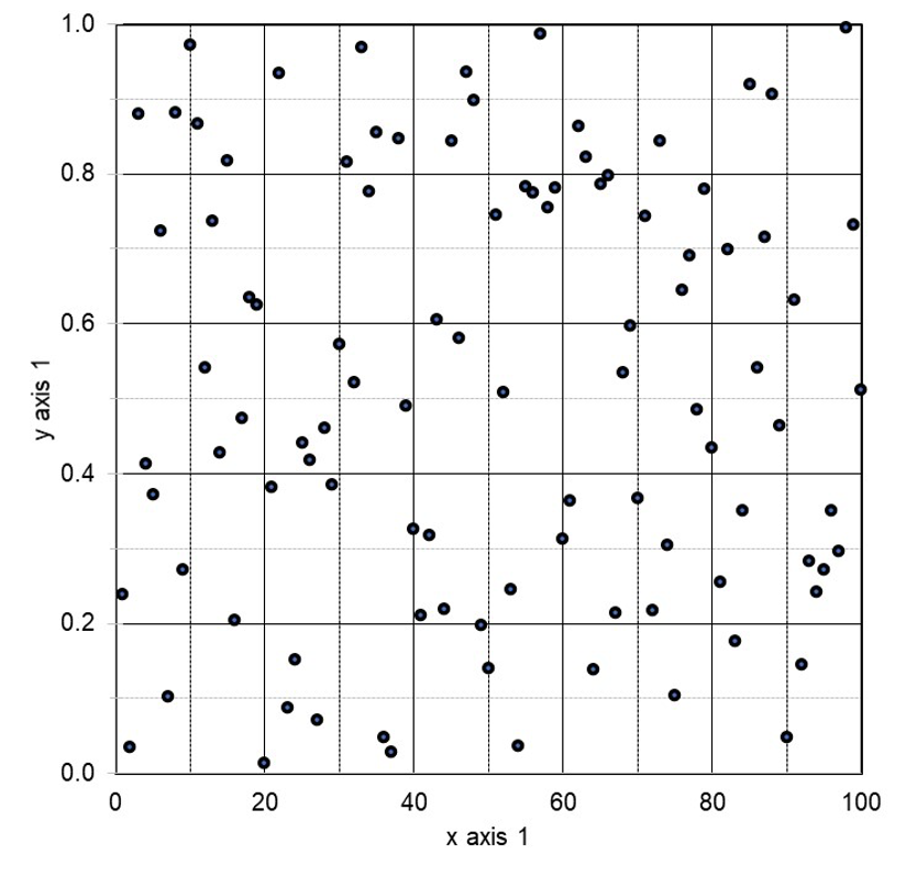
Figure A2.2: Rank order diagram of the same simulated series of 100 experiments designed to confirm or reject some unspecified null hypothesis

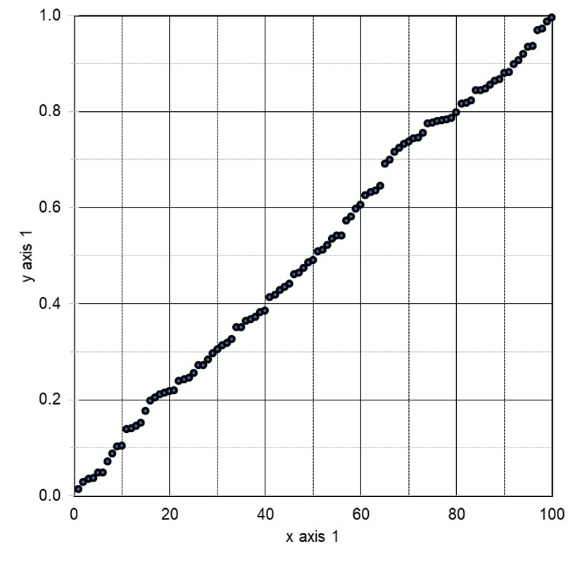
Appendix 3: Common Examples of Bilinear P-value Plot Behavior

Base studies ultimately selected for meta-analysis tend to be carefully screened and evaluated so that they are consistent in addressing a single research question of interest and that they meet other rigorous eligibility criteria regarding methods and datasets. Studies selected for meta-analyses are (supposed to be) directly comparable, basically homogeneous, so they can be aggregated. A p-value plot of meta-analysis data contains p-values drawn from carefully selected base studies all examining a single research claim—e.g., whether risk factor A causes disease B.

A p-value plot exhibiting bilinearity—two lines with very different slopes—ought not to exist in valid scientific literature. Such a p-value plot might be interpreted to mean that:

• for p-values < 0.05, the research claim is true—i.e., a true (positive) effect exists between risk factor A and disease B); or
• for p-values >0.05, the research claim is not true—i.e., a null (negative) effect exists between risk factor A and disease B).

Logically, both outcomes cannot be true. Widespread existence of p-hacking (which can be identified by counting) and publication bias support an interpretation that the research claim is not true.²⁰⁷ Confirmation bias is part of the process. Scientists making a research claim are required to back their claim up with strong evidence. They need to be able to explain away null findings (those carefully selected base studies with p-values >0.05). In science, one cannot “prove a negative” but a number of p-values on a 45-degree line is strong evidence that the negative effect is true.

Having stated this, bilinearity does not provide incontrovertible evidence of publication bias, p-hacking, or HARKing. Occasionally real effects will register as bilinear p-value plots—but this occurs rather rarely and can indicate an undetected and/or imperfectly controlled variable. Professionals and the public should take a bilinear p-value plot as a compelling reason to re-examine a field of literature for distorting biases. A given field’s conclusions should be regarded skeptically until the questions raised by a bilinear p-value plot have been resolved.

Three common examples of p-value plots of meta-analyses drawn from published literature that exhibit bilinear characteristics are provided. We should mention that our experience so far has been that most meta-analyses subjected to p-value plotting exhibit bilinearity. We strongly suspect that a disturbingly large portion of claims made in meta-analyses lack statistical support—although we cannot yet quantify that judgment.

Figure A3.1 plots the p-values of a meta-analysis of 23 RCTs that examined the mean difference in reduction of chronic low back pain at one month for spinal manipulative therapy (SMT) versus recommended therapies in adults older than 18 with chronic low back pain.²⁰⁸ The meta-analysis claimed that, “SMT produces similar effects to recommended therapies for chronic low back pain…”

Figure A3.1: P-value Plot, Meta-analysis of 23 RCT data sets, Mean difference in reduction of chronic low back pain at 1 month for spinal manipulative therapy (SMT) versus recommended therapies

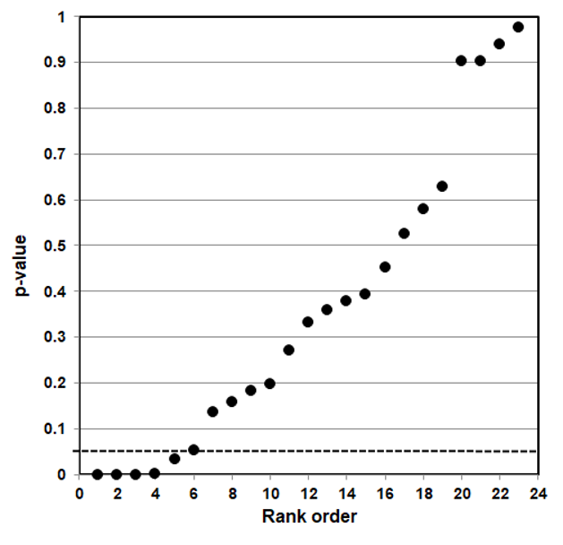
Figure A3.1 clearly depicts bilinear plot behavior. One cluster of small p-values follows a near-horizontal line—but most p-values, including several that are less than 0.05, approximately follow a 45-degree line. The pattern strongly suggests that publication bias, p-hacking, or HARKing has altered a field whose results supported the presumption of randomness—that there is no consistent overall positive association of spinal manipulative therapy and reduction in chronic low back pain compared to recommended therapies.

We note that in this instance the meta-analysis did not result in a false positive claim being made: Rubinstein et al. concluded that “SMT produces similar effects to recommended therapies for chronic low back pain.”²⁰⁹ The next two meta-analysis examples show similar bilinear p-value plot characteristics, however with likely false positive claims being made.

Figure A3.2 plots the p-values of a meta-analysis of 19 randomized clinical trials that examined the association between anxiety symptoms and omega-3 polyunsaturated fatty acids treatment compared with controls in varied populations.²¹⁰ This meta-analysis claimed that, “omega-3 PUFAs might help to reduce the symptoms of clinical anxiety.”

Figure A3.2: P-value Plot, Meta-analysis of 19 RCT data sets, Association of treatment with reduced anxiety symptoms in patients receiving and not receiving omega-3 polyunsaturated fatty acids

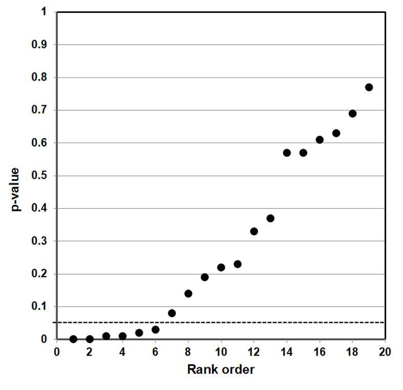
Figure A3.2 is similar to Figure A3.1, with p-values again taking a bilinear shape – a cluster of small p-values along the horizon, and most p-values approximately following a near 45 degree line. The pattern strongly suggests that publication bias, p-hacking, or HARKing has altered a field whose results supported the presumption of randomness—that there is no consistent overall positive association across the studies used in the meta-analysis.

In this instance, the meta-analysis registered a statistically significant association: “This review indicates that omega-3 PUFAs might help to reduce the symptoms of clinical anxiety.” The research field’s result had shifted not only in the direction of statistical significance, but across the line.

Figure A3.3 plots the p-values of a meta-analysis of 17 field observational studies examining the association between inferred exposure to PM_2.5 in ambient air and lung cancer incidence and mortality—16 cohort studies and one case-control study.²¹¹ This final meta-analysis made the following claim “Our findings suggest that long-term exposure to PM_2.5 is significantly associated both with LC [lung cancer] incidence and mortality.”

Figure A3.3: P-value Plot, Meta-analysis of 17 field observational data sets, Association between inferred exposure to PM_2.5 in ambient air and lung cancer incidence and mortality

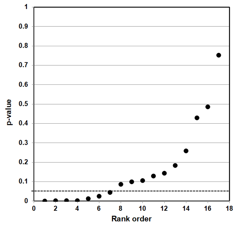
Figure A3.3 depicts bilinear plot behavior, with a cluster of small p-values on a nearly horizontal line and most p-values approximately following a 45-degree line. Although the data in Figure A3.3 are less clear than in Figure A3.1 and Figure A3.2, the distribution of the p-values from independent studies representing PM_2.5 in ambient air and lung cancer incidence and mortality clearly deviates from true nulls (Figure 4) or significant association (Figure 5). The curve forms an intermediate bow-shape rather than a 45-degree line (strong evidence of no significant association) or a horizontal line (strong evidence of a significant association).

The general pattern suggests that publication bias, p-hacking, or HARKing may have altered a field whose results, properly corrected, would indicate that there is no consistent overall positive association across the studies used in the meta-analysis. The evidence is mixed, but still strong enough to suggest that the claim of a significant association requires further investigation before it is accepted by researchers in the field.

Appendix 4: PM_2.5−Mortality Causality—Incomplete Evidence

Throughout this report we are addressing usual (typical) analysis methods used by researchers in the field of environmental epidemiology, accepting the data as given. We point out that multiple testing and multiple modeling (MTMM) problems are ignored and argue that any environmental epidemiology claims made without addressing MTMM problems lack sufficient statistical support.

We have not addressed other fundamental criticisms about the way environmental epidemiology researchers consider causality.²¹² For example, Cox recently provided an up-to-date summary of criticisms that continue to plague PM_2.5−mortality causality studies in environmental epidemiology, including:

• Omitted predictors and confounders.
• Uncontrolled residual confounding.
• Unmodeled interactions among variables.
• Untested and incorrect modeling assumptions.
• Unmodeled exposure uncertainties.
• Unjustified interventional causal interpretation of regression coefficients.²¹³

If you change a system, it should change in a predictable way. Classically, causality is established with experiments. Many factors are directly controlled, other factors are statistically controlled, and experimental units are assigned treatments at random. The entire process is preplanned and specified. After the experiment is run, the response of the system is examined. Absent full-scale experiments, so called quasi-experiments can provide information on causality.

Here we provide three examples of environmental epidemiology quasi-experiments that invalidate PM_2.5-mortality causal associations.²¹⁴

1. In 1970 the Clean Air Act Amendments designated U.S. counties with annual, average total suspended particulates (TSP) greater than a threshold as nonattainment locations. These nonattainment locations faced stricter regulations starting in 1972 than those in attainment locations. A natural experiment came into being with nonattainment and attainment counties forming two different groups.²¹⁵ The full data set covered 560 U.S. counties for six consecutive years (1969–1974) and was subjected to analysis comparing death rates in nonattainment to attainment counties. Air quality improved over the six years in nonattainment counties, but death rates did not. Using the same data, but a different analysis strategy, Obenchain came to the same conclusion and they also made the data set public.²¹⁶
2. In another noteworthy study, forest fires in Quebec in the summer of 2002 resulted in forest fire smoke migrating down the U.S. east coast.²¹⁷ PM_2.5 measurement data and mortality data were obtained for a 4-week period in July 2002 for Greater Boston (over 1.7 million people) and New York City (over 8 million people). Daily average PM_2.5 concentrations were noticeably increased in both cities for 3 days during this period—reaching as high as 63 μg/m^3 in Boston and 86 μg/m^3 in New York City versus 4–48 μg/m^3 in non-smoke days. Temporal patterns of natural-cause deaths and daily average PM_2.5 concentrations did not indicate any discernible increase in daily mortality in either city for high- versus non-smoke days.
3. Finally, Young studied and made public a data set containing daily deaths, daily air quality levels (PM_2.5 and ozone), daily temperature levels (minimum and maximum), and daily maximum relative humidity levels for the eight most populous California air basins.²¹⁸ The data set encompassed thirteen years, more than 2 million deaths and over 37,000 exposure days. The data set was analyzed using time series analysis. A sensitivity analysis was computed varying model parameters, locations and years—which included over 70,000 variations of analysis. The study found little evidence for association between air quality and deaths. Within the data set, there were several smoke/PM_2.5 events and they did not exhibit correlations with daily deaths.²¹⁹

Our MTMM critique does not depend on these questions of causality. Nevertheless, we also recommend that environmental epidemiology researchers and EPA regulators take account of this separate, serious causality critique.

Appendix 5: Supporting Information for Investigations of PM_2.5-Health Effect Association

All-cause mortality

We investigated the reliability of claims from studies used in meta-analysis associating PM_2.5 and other air quality components with all-cause mortality. We analyzed 29 risk ratios and confidence limits taken from 27 researchers for all-cause mortality and PM_2.5; two researchers had two papers. While other components were available for analysis, here we analyzed only results pertaining to PM_2.5 (see Figure A5.1).

Figure A5.1: Natural log of the Environmental Effect [Ln(EE)]and its Standard Error [SE Ln(EE)] for 29 Risk Ratios and Confidence Limits of PM_2.5−All-Cause Mortality Associations²²⁰

Rank	ID	Author	Year	Ln(EE)	SE Ln(EE)	Z value	p-value
1	337	Dai	2014	0.011731	0.001309	8.959154	3.27E-19
2	273	Chen	2011	0.004589	0.000558	8.219683	2.04E-16
3	758	Lee	2016	0.01548	0.001905	8.123914	4.51E-16
4	772	Li	2017	0.001699	0.000306	5.559715	2.7E-08
5	633	Janssen	2013	0.007968	0.002021	3.943442	8.03E-05
6	1774	Li	2018	0.002497	0.000661	3.776385	0.000159
7	1409	Tsai	2014	0.039268	0.010868	3.613243	0.000302
8	851	Madsen	2012	0.027615	0.00788	3.504571	0.000457
9	1733	Wu	2018	0.005485	0.001571	3.492337	0.000479
10	1714	Reyna	2012	0.008243	0.002527	3.261944	0.001107
11	489	Garret	2011	0.006678	0.002477	2.695497	0.007028
12	601	Hong	2017	0.112056	0.049633	2.257704	0.023964
13	245	Castillejos	2000	0.014692	0.007387	1.988796	0.046724
14	211	Burnett	2004	0.005993	0.003191	1.877872	0.060399
15	1691	Dockery	1992	0.017059	0.009617	1.773869	0.076085
16	84	Atkinson	2016	-0.01419	0.008234	-1.72311	0.084868
17	1691	Dockery	1992	0.022793	0.018614	1.224494	0.220766
18	975	Neuberger	2007	0.004988	0.005052	0.987326	0.323483
19	1709	Simpson	2000	0.007997	0.00815	0.981175	0.326506
20	974	Neuberger	2013	0.003992	0.004553	0.876757	0.380618
21	1695	Peters	2009	0.004888	0.006454	0.757427	0.448794
22	1411	Tsai	2014	0.007692	0.012302	0.625253	0.531805
23	748	Lanzinger	2016	-0.00404	0.006971	-0.57993	0.561965
24	59	Anderson	2001	0.00338	0.005955	0.567519	0.570362
25	827	Lopez-Villarrubia	2010	-0.00914	0.016166	-0.56548	0.571746
26	827	Lopez-Villarrubia	2010	-0.00682	0.016925	-0.40314	0.686842
27	186	Branis	2010	-0.002	0.006098	-0.3283	0.742686
28	120	Basagana	2015	0.001112	0.005225	0.212729	0.831538
29	722	Kollanus	2016	0.001998	0.041073	0.048645	0.961202

The claimed effect possessed a risk ratio of 1.0065, with 95% confidence limits of 1.0044 to 1.0086—that is, elevated PM_2.5 concentrations imposed a higher risk of all-cause mortality. A risk ratio of 1.000 is considered to register no effect; a risk ratio of 2.000 would provide evidence that elevated PM_2.5 concentrations imposed a higher risk of all-cause mortality; risk ratios between 1.000 and 2.000 indicate increasing evidence that elevated PM_2.5 concentrations impose a higher risk of all-cause mortality, from no effect to a strong effect.

So far as we know, a claim of 1.0065 is the smallest risk ratio claim for PM_2.5 that has been declared “real” in the literature. Indeed, to our knowledge, this is the smallest risk ratio claim which has ever been considered in anyscientific literature. So small a risk ratio indicates that even a small distortion in the base papers—whether from publication bias, HARKing, insufficient correction for MTMM, or other questionable research procedures—might have produced this “real” effect as a statistical artifact.

Heart attacks

We investigated the reliability of claims from studies used in meta-analysis of short-term air quality−heart attack associations. The number of outcomes, predictors, covariates and time lags available in each of the 34 studies were counted to estimate the number of statistical tests performed (Figure A5.2).

Figure A5.2: Outcomes, Predictors, and Lags in 34 studies, associations between air quality components and heart attacks²²¹

Citation #	Author	Outcomes	Predictors	Lags	Covariates	Space1	Space2	Space3
7	Braga	4	1	4	6	16	64	1,024
8	Koken	5	5	5	6	125	64	8,000
9	Barnett	7	5	1	10	35	1,024	35,840
10	Berglind	1	4	2	10	8	1,024	8,192
11	Cendon	2	5	8	5	80	32	2,560
12	Linn	3	4	3	8	36	256	9,216
19	Ye	8	5	5	3	200	8	1,600
20	Peters	1	8	2	11	16	2,048	32,768
21	Rich	1	5	6	9	30	512	15,360
22	Sullivan	4	4	3	8	48	256	12,288
23	Eilstein	1	12	6	5	72	32	2,304
24	Lanki	1	5	6	3	30	8	240
25	Mate	4	6	6	7	144	128	18,432
26	Medina	15	6	6	8	540	256	138,240
27	Poloniecki	7	5	1	5	35	32	1,120
28	Stieb	6	6	3	7	108	128	13,824
29	Zanobetti	5	2	3	11	30	2,048	61,440
30	Zanobetti	5	18	3	8	270	256	69,120
31	Zanobetti	5	2	2	9	20	512	10,240
32	Hoek	4	8	3	9	96	512	49,152
33	Cheng	1	5	3	6	15	64	960
34	Hsieh	1	5	3	6	15	64	960
35	Pope	1	2	7	13	14	8,192	114,688
36	D’Ippoliti	3	4	3	11	36	2,048	73,728
37	Henrotin	4	5	14	14	280	16,384	4,587,520
38	Ueda	3	1	3	7	9	128	1,152
39	Mann	4	4	7	9	112	512	57,344
40	Sharovsky	4	3	8	10	96	1,024	98,304
41	Belleudi	4	3	13	8	156	256	39,936
42	Nuvolone	1	3	8	9	24	512	12,288
43	Peters	4	5	4	10	80	1,024	81,920
44	Ruidavets	4	3	4	8	48	256	12,288
45	Zanobetti	2	6	3	7	36	128	4,608
46	Bhaskaran	1	5	7	7	25	128	3,200

We note that because these studies introduce statistical tests on lags, the number of Questions is no longer Outcomes x Predictors, but Outcomes x Predictors x Lags. Models = 2^k where k = number of Covariates. Search space = approximation of analysis search space = Questions x Models.²²²

Asthma

We investigated the reliability of claims from studies used in two meta-analyses of air quality−asthma attack associations: the first meta-analysis (Anderson) analyzed long-term cohort studies related to development of asthma and the second meta-analysis (Zheng) analyzed short-term time-series studies related to asthma attack.²²³

Causes and Risk factors

Asthma is associated with three principal characteristics: (1) variable airways obstruction, (2) airway hyperresponsiveness, and spasm with wheezing and coughing and (3) airway inflammation. Asthma may be characterized clinically by episodic, reversible obstruction of airways that variably presents as symptoms ranging from cough to wheezing, shortness of breath, or chest tightness.

The diagnosis of asthma/reactive airways is challenging. Asthma that starts young does not start in babies; it develops when victims are toddlers. Asthma that develops prior to the teen years may develop in hyperresponders (possessing an abnormally high degree of responsiveness) who would have benefited from desensitization due to lack of immune challenges in postneonatal immune system development. If adults who have smoked for a time develop bronchitis, they will demonstrate reactive airways that are triggered by various mechanisms—e.g., fumes, cold air, exercise—and so they may display the symptoms of late onset asthmatics.

There is even continuing debate as to whether asthma is one disease or several different diseases that include airway inflammation; however, two thirds (or more) of asthmatic patients have an allergic component to their disease and are thought to have allergic asthma. Not enough is currently known to rule out allergic causes in a vast majority of asthmatic problems.

As for development of asthma, the disease frequently first expresses itself early in the first few years of life, arising from a combination of genetic and non-genetic factors. Most investigators would agree there is a major hereditary contribution to the underlying causes of asthma and allergic diseases.²²⁴

Prevalence

We looked at asthma prevalence in the American (US) population in relation to ambient air quality. We accessed asthma prevalence data from the US Centers for Disease Control and Prevention (Atlanta, GA). The prevalence data we report here are from annual national surveys conducted by the National Center for Health Statistics (NCHS), the US Department of Health & Human Services, and are self-reported by respondents to the National Health Interview Survey. (Figure A5.3). Asthma prevalence in the US population increased from 4.2% in 1990 to 8% in 2006 and has since been relatively stable. Asthma prevalence in the US population was 7.9% in 2017.

We accessed US annual national air quality concentration averages over the same period (1990−2017) from the US Environmental Protection Agency. (Figure A5.4.). As shown in Figure A5.4, all air quality components of interest to the EPA declined (range 22−88%) over the 27−year period between 1990 and 2017.

In particular, US ambient NO₂ concentrations declined by 50% and PM_2.5 concentrations by 40% (2000−2017). Whereas prevalence of asthma in the US (population-weighted) increased by 88% during the same period. These conflicting trends suggest that other factors, rather than air quality components, may be more important in the development of asthma later in life.

Counts

Counts and analysis search spaces in 19 base studies of the first meta-analysis related to development of asthma are shown in Figure A5.5.

Figure A5.3: Annual prevalence of asthma in the US, population-weighted, 1990−2017 as reported by National Center for Health Statistics, National Health Interview Surveys²²⁵

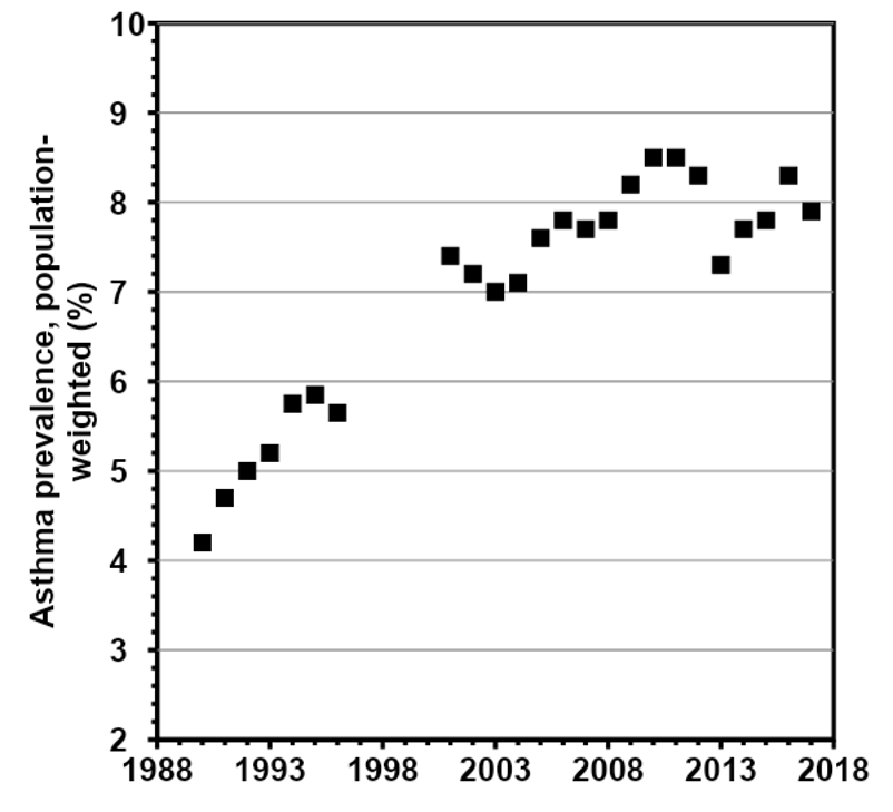
Figure A5.4: Change in US annual national air quality concentration averages and annual prevalence of asthma in the US (population-weighted) over the 27-year period 1990−2017 (except as noted)²²⁶

Parameter	Change
Nitrogen Dioxide (NO2) 1-Hour	−50%
Nitrogen Dioxide (NO2) Annual	−56%
Particulate Matter 2.5 microns (PM2.5) 24-Hour (2000−2017)	−40%
Particulate Matter 2.5 microns (PM2.5) Annual (2000−2017)	−41%
Particulate Matter 10 microns (PM10) 24-Hour (2010−2017)	−34%
Carbon Monoxide (CO) 8-Hour	−77%
Ozone (O3) 8-Hour	−22%
Sulfur Dioxide (SO2) 1-Hour	−88%
Prevalence of asthma	+88%

Figure A5.5: Counts and analysis search spaces in 19 base studies, associations between air quality components and development of asthma²²⁷

Study cohort	Outcomes	Predictors	Lags	Covariates	Questions	Models	Search space
BAMSE	7	3	4	6	84	64	5,376
British Columbia	1	8	4	7	32	128	4,096
CHS	1	2	8	15	16	32,768	524,288
CHS	1	6	5	10	30	1,024	30,720
CHS 2003	1	5	3	15	15	32,768	491,520
CHIBA	3	1	3	6	9	64	576
CHIBA	1	3	6	6	18	64	1,152
CHIBA	5	4	4	8	80	256	20,480
ECHRS	1	1	6	11	6	2,048	12,288
GINIplus+LISAplus	4	4	6	12	96	4,096	393,216
MISSEB	1	2	7	6	14	64	896
OLIN	1	3	4	5	3	32	96
OSLO	4	2	3	11	24	2,048	49,152
PIAMA	8	4	4	18	128	262,144	33,000,000
PIAMA	5	4	8	18	160	262,144	42,000,000
RHINE	1	2	1	8	2	256	512
TRAPCA	6	3	6	7	108	128	13,824
TRAPCA	7	3	4	9	84	512	43,008
AHSMOG	1	3	3	7	15	128	1,920

Counts and analysis search spaces in 34 base studies of the second meta-analysis related to asthma attack are shown in Figure A5.6.

Figure A5.6: Counts and analysis search spaces in 34 base studies, associations between air quality components and asthma attack²²⁸

Cit #	Author	Outcome	Predictor	Covariate	Lag	Space1	Space2	Space3
7	Braga	4	1	6	4	16	64	1,024
8	Koken	5	5	6	5	125	64	8,000
9	Barnett	7	5	10	1	35	1,024	35,840
10	Berglind	1	4	10	2	8	1,024	8,192
11	Cendon	2	5	5	8	80	32	2,560
12	Linn	3	4	8	3	36	256	9,216
19	Ye	8	5	3	5	200	8	1,600
20	Peters	1	8	11	2	16	2,048	32,768
21	Rich	1	5	9	6	30	512	15,360
22	Sullivan	4	4	8	3	48	256	12,288
23	Eilstein	1	12	5	6	72	32	2,304
24	Lanki	1	5	3	6	30	8	240
25	Mate´	4	6	7	6	144	128	18,432
26	Medina	15	6	8	6	540	256	138,240
27	Poloniecki	7	5	5	1	35	32	1,120
28	Stieb	6	6	7	3	108	128	13,824
29	Zanobetti	5	2	11	3	30	2,048	61,440
30	Zanobetti	5	18	8	3	270	256	69,120
31	Zanobetti	5	2	9	2	20	512	10,240
32	Hoek	4	8	9	3	96	512	49,152
33	Cheng	1	5	6	3	15	64	960
34	Hsieh	1	5	6	3	15	64	960
35	Pope	1	2	13	7	14	8,192	114,688
36	D’Ippoliti	3	4	11	3	36	2048	73,728
37	Henrotin	4	5	14	14	280	16,384	4,587,520
38	Ueda	3	1	7	3	9	128	1,152
39	Mann	4	4	9	7	112	512	57,344
40	Sharovsky	4	3	10	8	96	1,024	98,304
41	Belleudi	4	3	8	13	156	256	39,936
42	Nuvolone	1	3	9	8	24	512	12,288
43	Peters	4	5	10	4	80	1,024	81,920
44	Ruidavets	4	3	8	4	48	256	12,288
45	Zanobetti	2	6	7	3	36	128	4,608
46	Bhaskaran	1	5	7	5	25	128	3,200

In Figure A5.6: Space 1 = Outcomes x Predictors x Lags; Space 2 = 2^Covariates; Space 3 (analysis search space or number of statistical tests) = Space 1 x Space 2.

References

Acharjee M. K., Das, K., Young, S. S. In preparation. Air quality and lung cancer: Analysis via Local Control.

Akerlof, G. A., Michaillat, P. 2018. Persistence of false paradigms in low-power sciences. Proceedings of the National Academy of Sciences of the United States of America 115, 52: 13228–33. https://doi.org/10.1073/pnas.1816454115.

Allison, D. B., Brown, A. W., George, B. J., Kaiser, K. A. 2016. Reproducibility: A tragedy of errors. Nature 530, 7588: 27–29. https://doi.org/10.1038/530027a.

Altman, D, G. and Bland, J. M. 2011a. How to obtain a confidence interval from a P value. BMJ 343, d2090. https://doi.org/10.1136/bmj.d2090.

Altman, D. G. and Bland, J. M. 2011b. How to obtain the P value from a confidence interval. BMJ 343, d2304. https://doi.org/10.1136/bmj.d2304.

Anderson, H. R., Favarato, G., Atkinson, R. W. 2013. Long-term exposure to air pollution and the incidence of asthma: meta-analysis of cohort studies. Air Quality, Atmosphere & Health 6: 47–56. https://link.springer.com/article/10.1007/s11869-011-0144-5.

Anderson, M. S., Ronning, E. A., DeVries, R., Martinson, B. C. 2010. Extending the Mertonian norms: Scientists’ subscription to norms of research. The Journal of Higher Education 81, 3: 366–93. https://dx.doi.org/10.1353%2Fjhe.0.0095.

Archer, E. 2020. The intellectual and moral decline in academic research. The James G. Martin Center for Academic Renewal, January 29, 2020. https://www.jamesgmartin.center/2020/01/the-intellectual-and-moral-decline-in-academic-research/.

Bachmann, J. D. 2007. Will the circle be unbroken: A history of the US National Ambient Air Quality Standards. Journal of the Air & Waste Management Association 57, 6: 652–97. https://doi.org/10.3155/1047-3289.57.6.652.

Baker, M. 2016. 1,500 scientists lift the lid on reproducibility. Nature 533, 7604: 452–54. http://www.nature.com/news/1-500-scientists-lift-the-lid-on-reproducibility-1.19970.

Bandholm, T., Christensen, R., Thorborg, K., Trweek, S., Henriksen, M. 2017. Preparing for what the reporting checklists will not tell you: the PREPARE Trial guide for planning clinical research to avoid research waste. British Journal of Sports Medicine 51, 20: 1494–1501. https://doi.org/10.1136/bjsports-2017-097527.

Begley, C. G. and Ellis, L. M. 2012. Drug development: Raise standards for preclinical cancer research. Nature 483: 531–33. https://doi.org/10.1038/483531a.

Berger, J. O., Selke, T. 1987. Testing a point null hypothesis: the irreconcilability of p-values and evidence. Journal of the American Statistical Association 33, 112–22. https://doi.org/10.1080/01621459.1987.10478397.

Bidel, S., Hu, G., Jousilahti, P., Pukkala, E., Hakulinen, T., Tuomilehto, J. 2013. Coffee consumption and risk of gastric and pancreatic cancer—A prospective cohort study. International Journal of Cancer 132, 7: 1651–59. https://doi.org/10.1002/ijc.27773.

Blanton, H., Jaccard, J., Strauts, E., Mitchellm G., Tetlock. P. E. 2015. Toward a meaningful metric of implicit prejudice. The Journal of Applied Psychology 100, 5: 1468–81. https://doi.org/10.1037/a0038379.

Bowatte, G., Lodge, C., Lowe, A. J., Erbas, B., Perret, J., Abramson, M. J., Matheson, M., Dharmage, S. C. 2015. The influence of childhood traffic-related air pollution exposure on asthma, allergy and sensitization: a systematic review and a meta-analysis of birth cohort studies. Allergy 70, 3: 245–56. https://doi.org/10.1111/all.12561.

Briggs, W. 2016. Uncertainty The Soul of Modeling, Probability & Statistics. Switzerland: Springer International Publishing.

Briggs, W. M. 2017. The substitute for p-values. Journal of the American Statistical Association 112: 897-98. https://doi.org/10.1080/01621459.2017.1311264.

Briggs, W. M. 2019. Everything wrong with p-values under one roof. In Beyond Traditional Probabilistic Methods in Economics, ECONVN 2019, Studies in Computational Intelligence, Volume 809, eds. Kreinovich V., Thach N., Trung N., Van Thanh D. Cham, Switzerland: Springer. https://doi.org/10.1007/978-3-030-04200-4_2.

Bruns, S. B. and Ioannidis, J. P. A. 2016. P-curve and p-hacking in observational research. PloS One 11, 2: e0149144. https://doi.org/10.1371/journal.pone.0149144.

Buchanan, J. M. and Tullock, G. 2004. The Calculus of Consent: Logical Foundations of Constitutional Democracy. Indianapolis: Liberty Fund, Inc.

Calabrese, E. J. 2017. The mistaken birth and adoption of LNT: An abridged version. Dose-Response: A publication of International Hormesis Society 15, 4. https://doi.org/10.1177/1559325817735478.

Cao, J., Chow, J. C., Lee, F. S. C., Watson, J. G. 2013. Evolution of PM_2.5 measurements and standards in the U.S. and future perspectives for China. Aerosol and Air Quality Research 13, 4: 1197–1211. http://dx.doi.org/10.4209/aaqr.2012.11.0302.

Carlsson, R. and Agerström, J. 2016. A closer look at the discrimination outcomes in the IAT literature. Scandinavian Journal of Psychology 57, 4: 278–87. https://doi.org/10.1111/sjop.12288.

Carter, E. C., Schönbrodt, F. D., Gervais, W. M., Hilgard, J. 2019. Correcting for bias in psychology: A comparison of meta-analytic methods. Advances in Methods and Practices in Psychological Science 2, 2: 115–44. https://doi.org/10.1177/2515245919847196.

CASAC (Clean Air Scientific Advisory Committee). 2019. CASAC Review of the EPA’s Integrated Science Assessment for Particulate Matter (External Review Draft—October 2018). https://yosemite.epa.gov/sab/sabproduct.nsf/LookupWebReportsLastMonthCASAC/6CBCBBC3025E13B4852583D90047B352/%24File/EPA-CASAC-19-002+.pdf.

Case, R. B., Heller, S. S., Case, N. B., Moss, A. J. 1985. Type A behavior and survival after acute myocardial infarction. The New England Journal of Medicine 312, 12: 737–41. https://doi.org/10.1056/NEJM198503213121201.

Cecil, J. S., and Griffin, E. 1985. The role of legal policies in data sharing. In Sharing Research Data, eds. Fienberg, S.E., Martin, M. E., Straf, Miron L. Washington, D.C.: National Academy Press. 148–98. https://www.nap.edu/read/2033/chapter/15.

Chambers, C. 2017. The Seven Deadly Sins of Psychology, A Manifesto for Reforming the Culture of Scientific Practice. Princeton, NJ: Princeton University Press.

Chawla, D. S. 2020. Russian journals retract more than 800 papers after ‘bombshell’ investigation. Science, January 8, 2020. https://www.sciencemag.org/news/2020/01/russian-journals-retract-more-800-papers-after-bombshell-investigation.

Chay, K., Dobkin, C., Greenstone, M. 2003. The Clean Air Act of 1970 and adult mortality. Journal of Risk and Uncertainty 27, 3: 279–300. https://doi.org/10.1023/A:1025897327639.

Chen, D-G. and Peace, K. E. 2013. Applied Meta-Analysis with R. 2013. Boca Raton, FL: Chapman & Hall.

Clyde, M. 2000. Model uncertainty and health effects studies for particulate matter. Environmetrics. 11, 6: 745–63. https://doi.org/10.1002/1099-095X(200011/12)11:6<745::AID-ENV431>3.0.CO;2-N.

Cohen, J. 1994.The earth is round (p < .05). American Psychologist 49, 12: 997–1003. https://doi.org/10.1037/0003-066X.49.12.997.

Coleman. L. 2019. How to tackle the unfolding research crisis. Quillette, December 14, 2019. https://quillette.com/2019/12/14/how-to-tackle-the-unfolding-research-crisis/.

Cordes, C. 1998. Overhead Rates for Federal Research are as High as Ever, Survey Finds. The Chronicle of Higher Education, January 23, 1998. https://www.chronicle.com/article/Overhead-Rates-for-Federal/99293.

Coronado-Montoya, S., Levis, A. W., Kwakkenbos, L., Steele, R. J., Turner, E. H., Thombs, B. D. 2016. Reporting of positive results in randomized controlled trials of mindfulness-based mental health interventions. PLoS One 11, 4. https://doi.org/10.1371/journal.pone.0153220.

Cox, D. D. and Lee, J. S. 2008. Pointwise testing with functional data using the Westfall–Young randomization method. Biometrika 95, 3: 621–34. https://doi.org/10.1093/biomet/asn021.

Cox Jr., L. A. [Tony], Popken, D., Ricci, P. F. 2012. Temperature, not fine particulate Matter (PM2.5), is causally associated with short-term acute daily mortality rates: Results from one hundred United States cities. Dose-Response 11, 3: 319–43. https://doi.org/10.2203/dose-response.12-034.Cox.

Cox Jr., L.A. 2017. Do causal concentration–response functions exist? A critical review of associational and causal relations between fine particulate matter and mortality. Critical Reviews in Toxicology 47, 7: 609−37. https://doi.org/10.1080/10408444.2017.1311838.

Cox Jr., L.A. Popkin, D. A., Sun, Richard X. 2018. Causal Analytics for Applied Risk Analysis. Cham, Switzerland: Springer.

Cox Jr., L. A. 2020. Letter to the Editor. Causal effects of air pollution on mortality rate in Massachusetts. American Journal of Epidemiology, September 2020. https://doi.org/10.1093/aje/kwaa186.

Crandall, C. S. and Sherman, J. W. 2016. On the scientific superiority of conceptual replications for scientific progress. Journal of Experimental Social Psychology 66: 93–99. http://dx.doi.org/10.1016/j.jesp.2015.10.002.

Cuff, M. 2016. Shipping industry agrees to cap sulphur emissions by 2020. The Guardian. https://www.theguardian.com/environment/2016/oct/28/shipping-industry-agrees-to-cap-sulphur-emissions-by-2020.

Curb, J. D., Hardy, R. J., Labarthe, D. R., Borhani, N. O., Taylor, J. O. 1982. Reserpine and breast cancer in the Hypertension Detection and Follow-Up Program. Hypertension 4, 2: 307–11. https://doi.org/10.1161/01.HYP.4.2.307.

De Souto Barreto, P., Rolland, Y., Vellas, B., Maltais, M. 2019. Association of Long-term Exercise Training with Risk of Falls, Fractures, Hospitalizations, and Mortality in Older Adults: A systematic Review and Meta-analysis. JAMA Internal Medicine 179, 3: 394–405. https://doi.org/10.1001/jamainternmed.2018.5406.

De Vrieze, J. 2018. Meta-analyses were supposed to end scientific debates. Often, they only cause more controversy. Science, September 18, 2018. https://www.sciencemag.org/news/2018/09/meta-analyses-were-supposed-end-scientific-debates-often-they-only-cause-more.

Dickersin, K., Chan, S., Chalmers, T. C., Sacks, H. S., Smith, H., Jr. 1987. Publication bias and clinical trials. Controlled Clinical Trials 8, 4: 343–53. https://doi.org/10.1016/0197-2456(87)90155-3.

Dockery, D. W., Pope III, C. A., Xu, X., Spengler, J. D., Ware, J. H., Fay, M. E., Ferris, B. G., Speizer, F. E. 1993. An association between air pollution and mortality in six U.S. cities. New England Journal of Medicine 329: 1753–59. https://doi.org/10.1056/nejm199312093292401.

Dooley, D., Fielding, J., Levi, L. 1996. Health and Unemployment. Annual Review of Public Health 17: 449−65. https://doi.org/10.1146/annurev.pu.17.050196.002313.

DOJ (Department of Justice). 2016. Department of Justice Announces New Department-Wide Implicit Bias Training for Personnel. Office of Public Affairs, The United States Department of Justice, June 27, 2016. https://www.justice.gov/opa/pr/department-justice-announces-new-department-wide-implicit-bias-training-personnel.

Edwards, M. A. and Roy, S. 2017. Academic research in the 21st century: Maintaining scientific integrity in a climate of perverse incentives and hypercompetition. Environmental Engineering Science 34, 1: 51–61. https://dx.doi.org/10.1089%2Fees.2016.0223.

Engber, D. 2017. Daryl Bem proved ESP Is real. Which means science is broken. Slate, June 7, 2017. https://slate.com/health-and-science/2017/06/daryl-bem-proved-esp-is-real-showed-science-is-broken.html.

Enstrom, J. E. 2005. Fine particulate air pollution and total mortality among elderly Californians, 1973–2002. Inhalation Toxicology 17, 14: 803–816. https://doi.org/10.1080/08958370500240413.

Enstrom, J. E. 2017. Fine particulate matter and total mortality in Cancer Prevention Study cohort reanalysis. Dose Response 15, 1: 1–12. https://doi.org/10.1177/1559325817693345.

EPA (Environmental Protection Agency). 2011. EPA Report Underscores Clean Air Act’s Successful Public Health Protections/Landmark law saved 160,000 lives in 2010 alone. United States Environmental Protection Agency,
https://archive.epa.gov/epapages/newsroom_archive/newsreleases/f8ad3485e788be5a8525784600540649.html.

EPA (Environmental Protection Agency). N.D. Good Laboratory Practices Standards Compliance Monitoring Program. Compliance. United States Environmental Protection Agency. Accessed August 14, 2020. https://www.epa.gov/compliance/good-laboratory-practices-standards-compliance-monitoring-program.

Erikssen, J., Thaulow, E., Stormorken, H., Brendemoen, O., Hellem, A. 1980. AB0 blood groups and coronary heart disease (CHD). Thrombosis and Haemostasis 43, 2: 137–40. https://doi.org/10.1055/s-0038-1650035.

Fanelli, D. 2009. How many scientists fabricate and falsify research? A systematic review and meta-analysis of survey data. PLoS One 4, 5: e5738. https://doi.org/10.1371/journal.pone.0005738.

Fanelli, D. 2018. Opinion: Is science really facing a reproducibility crisis, and do we need it to? Proceedings of the National Academy of Sciences of the United States of America 115, 11: 2628–31. https://doi.org/10.1073/pnas.1708272114.

Faruque, S., Tong, J., Lacmanovic, V., Agbonghae, C., Minaya, D. M., Czaja, K. 2019. The dose makes the poison: Sugar and obesity in the United States—a review. Polish Journal of Food and Nutrition Sciences 69, 3: 219–33. https://doi.org/10.31883/pjfns/110735.

Favarato, G., Anderson, H. R., Atkinson, R., Fuller, G., Mills, I., Walton, H. 2014. Traffic-related pollution and asthma prevalence in children. Quantification of associations with nitrogen dioxide. Air Quality, Atmosphere, & Health 7, 4: 459–66. https://doi.org/10.1007/s11869-014-0265-8.

Feinstein, A. R. 1988. Scientific standards in epidemiologic studies of the menace of daily life. Science 242: 1257–63. https://doi.org/10.1126/science.3057627.

Fisher R. A. 1925. Statistical Methods for Research Workers. Edinburgh: Oliver and Boyd. https://www.scribd.com/document/58873576/Fisher-R-a-1925-Statistical-Methods-for-Research-Workers.

Fisher R. A. 1935. The logic of inductive inference. Journal of the Royal Statistical Society 98, 1: 39–82.https://www.jstor.org/stable/pdf/2342435.pdf?seq=1.

Franco, A., Malhotra, N., Simonovits, G. 2014. Publication bias in the social sciences: Unlocking the file drawer. Science 345: 1502–05. https://doi.org/10.1126/science.1255484.

Freese, J. and Peterson, D. 2018. The emergence of statistical objectivity: Changing ideas of epistemic vice and virtue in science. Sociological Theory 36, 3: 289–313, https://doi.org/10.1177/0735275118794987.

Friedman, M. and Rosenman, R. H. 1959. Association of specific overt behaviour pattern with blood and cardiovascular findings: blood cholesterol level, blood clotting time, incidence of arcus senilis, and clinical coronary artery disease. Journal of the American Medical Association 169, 12: 1286–96. http://dx.doi.org/10.1001/jama.1959.03000290012005.

Gal, T. S., Tucker, T. C., Gangopadhyay, A., Chen, Z. 2014. A data recipient centered de-identification method to retain statistical attributes. Journal of Biomedical Informatics 50: 32–45. https://doi.org/10.1016/j.jbi.2014.01.001.

Garrison, R. J., Havlik, R. J., Harris, R. B., Feinleib, M., Kannel, W. B., Padgett, S. J. 1976. ABO blood group and cardiovascular disease: the Framingham study. Atherosclerosis 25, 2–3: 311–318. https://doi.org/10.1016/0021-9150(76)90036-8.

Ge, Y., Dudoit, S., Speed, T. P. 2003. Resampling-based multiple testing for microarray data analysis. Technical Report #633: 1–41. https://statistics.berkeley.edu/sites/default/files/tech-reports/633.pdf.

Gelman, A. and Greenland, S. 2019. Are confidence intervals better termed “uncertainty intervals”? BMJ (Clinical research ed.) 366: l5381. https://doi.org/10.1136/bmj.l5381.

Gerber, A. S. and Malhotra, N. 2008. Publication bias in empirical sociological research do arbitrary significance levels distort published results? Sociological Methods and Research 37, 1: 3–30. https://doi.org/10.1177/0049124108318973.

Glaeser, E.L. 2006. Researcher incentives and empirical methods. NBER Technical Working Papers 0329, National Bureau of Economic Research, Inc. https://www.nber.org/papers/t0329.pdf.

Glass, G. V. 1976. Primary, secondary, and meta-analysis of research. Educational Researcher 5, 10: 3–8.https://doi.org/10.3102/0013189X005010003.

Gobry, P.-E. 2016. Big Science is Broken. The Week, April 18, 2016. https://theweek.com/articles/618141/big-science-broken.

Gold, M. S. 2020. The role of alcohol, drugs, and deaths of despair in the U.S.’s falling life expectancy. Missouri Medicine 117, 2: 99–101. https://www.ncbi.nlm.nih.gov/pubmed/32308224.

Goldacre, M. J. 1993. Cause-specific mortality: understanding uncertain tips of the disease iceberg. Journal of Epidemiology and Community Health 47, 6: 491–496. https://doi.org/10.1136/jech.47.6.491.

Goodman, S. N., Fanelli, D., Ioannidis, J. P. A. 2016. What does research reproducibility mean? Science Translational Medicine 8, 341: 1–6. https://doi.org/10.1126/scitranslmed.aaf5027.

Greenwald, A. G. 1975. Consequences of prejudice against the null hypothesis. Psychological Bulletin 82, 1: 1–20. https://doi.org/10.1037/h0076157.

Greven, S., Dominici, F., Zeger, S. 2011. An approach to the estimation of chronic air pollution effects using spatio-temporal information. Journal of the American Statistical Association 106, 494: 396–406. https://doi.org/10.1198/jasa.2011.ap09392.

Grimes, D. R., Bauch, C. T., Ioannidis, J. 2018. Modelling science trustworthiness under publish or perish pressure. Royal Society Open Science 5, 1: 171511. https://doi.org/10.1098/rsos.171511.

Grossman, J. and Mackenzie, F. J. 2005. The Randomized Controlled Trial: gold standard, or merely standard? Perspectives in Biology and Medicine 48, 4: 516–34. https://doi.org/10.1353/pbm.2005.0092.

GS (Google Scholar). 2020a. https://scholar.google.com/scholar_lookup?hl=en-US&publication_year=1993&author=+Westfall+PHauthor=+Young+SS&title=Resampling-based+multiple+testing%3A+examples+and+methods+for+p-value+adjustment, October 8, 2020.

GS (Google Scholar). 2020b. https://scholar.google.com/scholar?hl=en&as_sdt=5%2C33&sciodt=0%2C33&cites=2910987059377145085&scipsc=1&q=%22environmental+health+perspectives%22&btnG=, October 8, 2020.

Halsey, L. G., Curran-Everett, D., Vowler, S. L., Drummond, G. B. 2015. The fickle P value generates irreproducible results. Nature Methods 12, 3: 179–85. https://doi.org/10.1038/nmeth.3288.

Harris, R. 2017. Rigor Mortis: How Sloppy Science Creates Worthless Cures, Crushes Hope, and Wastes Billions. New York, NY: Basic Books.

Hartgerink, C. H. J. 2017. “Reanalyzing Head et al. (2015): investigating the robustness of widespread p-hacking. PeerJ 5, e3068. https://doi.org/10.7717/peerj.3068.

Hayat, M. J., Powell, A., Johnson, T., Cadwell, B. L. 2017. Statistical methods used in the public health literature and implications for training of public health professionals. PLoS One 12, 6: e0179032. https://doi.org/10.1371/journal.pone.0179032

Head, M. L., Holman L., Lanfear, R., Kahn, A. T., Jennions, M. D. 2015. The extent and consequences of p-hacking in science. PLoS Biology 13, 3: e1002106. https://doi.org/10.1371/journal.pbio.1002106.

Heinonen, O. P., Shapiro, S., Tuominen, L., Turunen, M. I. 1974. Reserpine use in relation to breast cancer. Lancet (London, England), 2(7882), 675–77. https://doi.org/10.1016/s0140-6736(74)93259-0.

Hennen, A. 2019. The Credibility Issue in Nutrition Science is a Sign for All of Higher Ed. The James G. Martin Center for Academic Renewal, November 27, 2019. https://www.jamesgmartin.center/2019/11/the-credibility-issue-in-nutrition-science-is-a-sign-for-all-of-higher-ed/.

Herold, E. 2018. Researchers Behaving Badly: Known Frauds Are “the Tip of the Iceberg.” Leapsmag. October 19, 2018. https://leapsmag.com/researchers-behaving-badly-why-scientific-misconduct-may-be-on-the-rise/.

Huang, F., Pan, B., Wu, J., Chen, E., Chen, L. 2017. Relationship between exposure to PM2.5 and lung cancer incidence and mortality: A meta-analysis. Oncotarget 8, 26: 43322–43331. https://doi.org/10.18632/oncotarget.17313.

Hubbard, R. 2015. Corrupt Research: The Case for Reconceptualizing Empirical Management and Social Science. London, UK: Sage Publications.

IMO (International Maritime Organization). 2020. Sulphur 2020—cutting sulphur oxide emissions. IMO, London, UK. http://www.imo.org/en/MediaCentre/HotTopics/Pages/Sulphur-2020.aspx.

Ioannidis, J. P. A. 2005. Why most published research findings are false. PLoS Medicine 2, 8: e124. https://doi.org/10.1371/journal.pmed.0020124.

Ioannidis, J. P., Tarone, R., McLaughlin, J. K. 2011. The false-positive to false-negative ratio in epidemiologic studies. Epidemiology 22, 4: 450–56. https://doi.org/10.1097/EDE.0b013e31821b506e.

Ioannidis, J. P. A. 2016. The mass production of redundant, misleading, and conflicted systematic reviews and meta-analyses. The Milbank Quarterly 94, 3: 485–514. https://doi.org/10.1111/1468-0009.12210.

IQA (Information Quality Act). 2000. Sec. 515, Treasury and General Government Appropriations Act for Fiscal Year 2001 (Public Law 106-554), https://www.fws.gov/informationquality/section515.html.

ISAPM (Integrated Science Assessment For Particulate Matter). 2009. U.S. EPA. Integrated Science Assessment (ISA) For Particulate Matter (Final Report, Dec 2009). U.S. Environmental Protection Agency, Washington, DC, EPA/600/R-08/139F. https://cfpub.epa.gov/ncea/risk/recordisplay.cfm?deid=216546.

Jaeger, R. G. and Halliday, T. R. 1998. On confirmatory versus exploratory research. Herpetologica 54, Supplement: S64–S66. https://www.jstor.org/stable/3893289?seq=1.

Janes, H., Dominici, F., Zeger, S. 2007. Trends in air pollution and mortality: An approach to the assessment of unmeasured confounding. Epidemiology 18, 4: 416–23. https://doi.org/10.1097/ede.0b013e31806462e9.

John, L. K., Loewenstein, G., Prelec, D. 2012. Measuring the prevalence of questionable research practices with incentives for truth telling. Psychological Science 23, 5: 524–32. https://doi.org/10.1177/0956797611430953.

Jones, D., Molitor, D., Reif, J. 2019a. What Do Workplace Wellness Programs Do? Evidence from the Illinois Workplace Wellness Study. The Quarterly Journal of Economics 134, 4: 1747–91.https://doi.org/10.1093/qje/qjz023.

Jones, D., Molitor, D., Reif, J. 2019b. Documentation for Illinois Workplace Wellness Study. https://www.nber.org/workplacewellness/s/wyoung.pdf.

Joseph, A. 2020. Lancet, New England Journal retract Covid-19 studies, including one that raised safety concerns about malaria drugs. Statnews, June 4, 2020. https://www.statnews.com/2020/06/04/lancet-retracts-major-covid-19-paper-that-raised-safety-concerns-about-malaria-drugs/.

Kaiser, J. 2017. NIH plan to reduce overhead payments draws fire. Science, June 2, 2017.https://www.sciencemag.org/news/2017/06/nih-plan-reduce-overhead-payments-draws-fire.

Keller, V. 2015. Knowledge and the Public Interest, 1575-1725. Cambridge, MA: Cambridge University Press.

Kim, S. Y. and Kim, Y. 2018. The ethos of science and its correlates: An empirical analysis of scientists’ endorsement of Mertonian norms. Science, Technology, and Society, 23, 1: 1–24. https://doi.org/10.1177/0971721817744438.

Kindzierski, W., Young, S. S., Meyer, T., Dunn, J. In preparation. Evaluation of a meta-analysis of ambient air quality as a risk factor for asthma exacerbation. https://arxiv.org/abs/2010.08628 [stat.AP].

Krewski, D., Burnett, R. T., Goldberg, M. S., Goldberg, M. S., Hoover, K., Siemiatycki, J., Jerrett, M., Abrahamowicz, M., White, W. H. 2000. Reanalysis of the Harvard Six Cities Study and the American Cancer Society Study of Particulate Air Pollution and Mortality. Special Report. Cambridge, MA: Health Effects Institute.https://www.healtheffects.org/publication/reanalysis-harvard-six-cities-study-and-american-cancer-society-study-particulate-air.

Kühberger, A., Fritz, A., Scherndl, T. 2014. Publication bias in psychology: A diagnosis based on the correlation between effect size and sample size. PLoS One 9, 9: e105825. https://doi.org/10.1371/journal.pone.0105825.

Kuhn, E. 2016. Science And Deference: The “Best Available Science” Mandate is A Fiction in the Ninth Circuit. Harvard Environmental Law Review, November 7, 2016. https://harvardelr.com/2016/11/07/elrs-science-and-deference-the-best-available-science-mandate-is-a-fiction-in-the-ninth-circuit/.

Kushida, C. A., Nichols, D. A., Jadrnicek, R., Miller, R., Walsh, J. K., Griffin, K. 2012. Strategies for de-identification and anonymization of electronic health record data for use in multicenter research studies. Medical Care 50 Suppl (Suppl): S82–S101. https://doi.org/10.1097/MLR.0b013e3182585355.

Kweon, S., Kim, Y., Jang, M-j., Kim, Y., Kim, K., Choi, S., Chun, C., Khang, Y-H., Oh, K. 2014. Data resource profile: The Korea National Health and Nutrition Examination Survey (KNHANES). International Journal of Epidemiology 43, 1: 69–77. https://doi.org/10.1093/ije/dyt228.

Labarthe, D. R. and O’Fallon, W. M. 1980. Reserpine and breast cancer. A community-based longitudinal study of 2,000 hypertensive women. Journal of the American Medical Association 243, 22: 2304–10. https://jamanetwork.com/journals/jama/article-abstract/370217.

Lander, E. and Kruglyak, L. 1995. Genetic dissection of complex traits: guidelines for interpreting and reporting linkage results. Nature Genetics 11, 3: 241–47. https://doi.org/10.1038/ng1195-241.

Lee, P. N., Forey, B. A., Coombs, K. J. 2012. Systematic review with meta-analysis of the epidemiological evidence in the 1900s relating smoking to lung cancer. BMC Cancer 12, 385. https://doi.org/10.1186/1471-2407-12-385.

Leslie, I. 2016. The sugar conspiracy. The Guardian, April 7, 2016. https://www.theguardian.com/society/2016/apr/07/the-sugar-conspiracy-robert-lustig-john-yudkin.

Lhamon, C. E. 2016. Dear Colleague Letter: Preventing Racial Discrimination in Special Education. Office for Civil Rights, United States Department of Education, December 12, 2016. https://www2.ed.gov/about/offices/list/ocr/letters/colleague-201612-racedisc-special-education.pdf.

Li, X., Huang, S., Jiao, A., Yang, X., Yun, J., Wang, Y., Xue, X., Chu, Y., Liu, F., Liu, Y., Ren, M., Chen, X., Li, N., Lu, Y., Mao, Z., Tian, L., Xiang, H. 2017. Association between ambient fine particulate matter and preterm birth or term low birth weight: An updated systematic review and meta-analysis. Environmental Pollution 227: 596–605. https://doi.org/10.1016/j.envpol.2017.03.055.

Lilienfeld, S. O. 2017. Psychology’s replication crisis and the grant culture: Righting the ship. Perspectives on Psychological Science 12, 4: 660–64. https://doi.org/10.1177/1745691616687745.

Lorenc, T., Felix, L., Petticrew, M., Melendez-Torres, G. J., Thomas, J., Thomas, S., O’Mara-Eves, A., Richardson, M. 2016. Meta-analysis, complexity, and heterogeneity: a qualitative interview study of researchers’ methodological values and practices. Sytematic Reviews 5, 1: 192. https://doi.org/10.1186/s13643-016-0366-6.

MacMahon, B., Yen, S., Trichopoulos, D., Warren, K., Nardi, G. 1981. Coffee and cancer of the pancreas. New England Journal of Medicine 304: 630–33. https://doi.org/10.1056/nejm198103123041102.

Manuel, T. 2019. Why the way we use statistical significance has created a crisis in science. Science: The Wire, March 31, 2019. https://science.thewire.in/the-sciences/why-the-way-we-use-statistical-significance-has-created-a-crisis-in-science/.

Martino, J. P. 2017. Science Funding: Politics and Porkbarrel. New York, NY: Routledge.

Mathews, F., Johnson, P. J., Neil, A. 2008. You are what your mother eats: evidence for maternal preconception diet influencing foetal sex in humans. Proceedings of the Royal Society B: Biological Sciences 275, 1643: 1661–68.https://dx.doi.org/10.1098%2Frspb.2008.0105.

Mathews, F., Johnson, P. J., Neil, A. 2009. Reply to Comment by Young et al. Proceedings of the Royal Society B: Biological Sciences 276, 1660: 1213–14. https://doi.org/10.1098/rspb.2008.1781.

Mayes, L. C., Horwitz, R. I., Feinstein, A. R. 1988. A collection of 56 topics with contradictory results in case-control research. International Journal of Epidemiology 17, 3: 680–85. https://doi.org/10.1093/ije/17.3.680.

Mayo, D. M. 2018. Statistical Inference as Severe Testing: How to Get Beyond the Statistics Wars. Cambridge, MA: Cambridge University Press.

McCambridge, J. 2007. A case study of publication bias in an influential series of reviews of drug education. Drug and Alcohol Review 26, 5: 463–68. https://doi.org/10.1080/09595230701494366.

McCormack, J., Vandermeer, B., Allan, G. M. 2013. How confidence intervals become confusion intervals. BMC Medical Research Methodology 13, 134. https://doi.org/10.1186/1471-2288-13-134.

McKie, R. 2016. The Life Project by Helen Pearson review—scientific marvel of the everyman. The Guardian, February 28, 2016. https://www.theguardian.com/science/2016/feb/28/the-life-project-helen-pearson-review-cohort-study.

Meach, R. 2018. From John Yudkin to Jamie Oliver: A short but sweet history on the war against sugar. In Proteins, Pathologies and Politics: Dietary Innovation and Disease from the Nineteenth Century, eds. Gentilcore, D. and Smith, M. London and New York: Bllomsbury Academic. Chapter 7. https://www.ncbi.nlm.nih.gov/books/NBK542158/.

Mehta, S., Shin, H., Burnett, R., North, T., Cohen, A. J. 2013. Ambient particulate air pollution and acute lower respiratory infections: a systematic review and implications for estimating the global burden of disease. Air Quality, Atmosphere, & Health 6, 1: 69–83. https://doi.org/10.1007/s11869-011-0146-3.

Meinshausen, N. Maathuis, M. H., Bühlmann, P. 2011. Asymptotic optimality of the Westfall--Young permutation procedure for multiple testing under dependence. Annals of Statistics 39, 6: 3369–91.https://projecteuclid.org/euclid.aos/1330958683.

Merton, R. K. 1973. The Sociology of Science: Theoretical and Empirical Investigations. Chicago, IL: The University of Chicago Press.

Michaels, P. J. 2008. Evidence for “publication bias” concerning global warming in Science and Nature. Energy & Environment 19, 2: 287–301. https://doi.org/10.1260/095830508783900735.

Milloy, S. J. 2016. Scare Pollution: Why and How to Fix the EPA. USA: Bench Press.

Milojevic, A., Wilkinson, P., Armstrong, B., Bhaskaran, K., Smeeth, L., Hajat, S. 2014. Short-term effects of air pollution on a range of cardiovascular events in England and Wales: Case-crossover analysis of the MINAP database, hospital admissions and mortality. Heart (British Cardiac Society) 100, 14: 1093−98. https://doi.org/10.1136/heartjnl-2013-304963.

Montgomery, D. C. and Runger, G. C. 2003 Applied Statistics and Probability for Engineers. New York: John Wiley & Sons.

Moolgavkar, S. H., Luebeck, E. G., Hall, T. A., Anderson, E. L. 1995. Particulate air pollution, sulfur dioxide, and daily mortality: A reanalysis of the Steubenville data. Inhalation Toxicology 7, 1: 35–44. https://doi.org/10.3109/08958379509014269.

Moolgavkar, S. H., McClellan, R. O., Dewanji, A., Turim, J., Luebeck, E. G., Edwards, M. 2013. Time-series analyses of air pollution and mortality in the United States: A subsampling approach. Environmental Health Perspectives121, 1: 73–78. https://doi.org/10.1289/ehp.1104507.

Mustafic, H., Jabre P., Caussin, C., Murad, M. H., Escolano, S., Tafflet, M., Périer, M.-C., Marijon, E., Vernerey, D., Empana, J.-P., Jouven, X. 2012. Main air pollutants and myocardial infarction: A systematic review and meta-analysis. Journal of the American Medical Association 307, 7: 713−21. https://doi.org/10.1001/jama.2012.126.

NASEM (National Academies of Sciences, Engineering, and Medicine). 1991. Environmental Epidemiology, Volume 1: Public Health and Hazardous Wastes. Washington, DC: The National Academies Press. https://doi.org/10.17226/1802.

NASEM (National Academies of Sciences, Engineering, and Medicine). 2016. Statistical Challenges in Assessing and Fostering the Reproducibility of Scientific Results: Summary of a Workshop. Washington, DC: The National Academies Press. https://www.nap.edu/read/21915/.

NASEM (National Academies of Science, Engineering, and Medicine). 2019. Reproducibility and Replicability in Science. Washington, D.C.: The National Academies Press. https://www.nap.edu/read/25303/.

NCHS (National Center for Health Statistics). 2008. Prevalence of overweight, obesity and extreme obesity among adults: United States, trends 1976-80 through 2005-2006. Health E-Stats. https://www.cdc.gov/nchs/data/hestat/overweight/overweight_adult.htm.

NDSR (National Diabetes Statistics Report). 2020. National Diabetes Statistics Report 2020. Estimates of Diabetes and Its Burden in the United States. Centers for Disease Control and Prevention, U.S. Department of Health and Human Services.

Nemery, B., Hoet, P. H. M., Nemmar, A. 2001. The Meuse Valley fog of 1930: an air pollution disaster. Lancet 357, 9257: 704−08. https://doi.org/10.1016/s0140-6736(00)04135-0.

Nilsen, E. B., Bowler, D. E., Linnell, J. D. C. 2020. Exploratory and confirmatory research in the open science era. Journal of Applied Ecology 57, 4: 842−47. https://doi.org/10.1111/1365-2664.13571.

Nissen, S. B., Magidson, T., Gross, K., Bergstrom, C. T. 2016. Publication bias and the canonization of false facts. eLife5: e21451. https://doi.org/10.7554/elife.21451.

Nosek, B. and Errington, T. M. 2020. What is replication? PloS Biology 18, 3: e3000691.https://doi.org/10.1371/journal.pbio.3000691.

Obenchain, R. and Young, S. S. 2017. Local Control strategy: Simple analyses of air pollution data can reveal heterogeneity in longevity outcomes. Risk Analysis 37: 1742−53. https://doi.org/10.1111/risa.12749.

Ogden, T. 2011. Lawyers beware! The scientific process, peer review, and the use of papers in evidence. The Annals of Occupational Hygiene 55, 7: 689–691. https://doi.org/10.1093/annhyg/mer056.

Olson, C.M., Rennie, D., Cook, D., Dickersin, K., Flanagin, A., Hogan, J. W., Zhu, Q., Reiling, J., Pace, B. 2002. Publication bias in editorial decision making. Journal of the American Medical Association 287, 21: 2825–2828. https://doi.org/10.1001/jama.287.21.2825.

OMB (Office of Management and Budget). 2019. Improving Implementation of the Information Quality Act. https://www.whitehouse.gov/wp-content/uploads/2019/04/M-19-15.pdf.

Open Science Collaboration [Brian Nosek, et al.]. 2015. Estimating the reproducibility of psychological science. Science 349, 6251: aac4716. https://doi.org/10.1126/science.aac4716.

Orellano, P., Reynoso, J., Quaranta, N., Bardach, A., Ciapponi, A. 2020. Short-term exposure to particulate matter (PM₁₀ and PM_2.5), nitrogen dioxide (NO₂), and ozone (O₃) and all-cause and cause-specific mortality: Systematic review and meta-analysis. Environment International 142: 105676. https://doi.org/10.1016/j.envint.2020.105876.

Oreskes, N. and Conway, E. M. 2010. Merchants of Doubt: How a Handful of Scientists Obscured the Truth on Issues from Tobacco Smoke to Global Warming. New York, NY: Bloomsbury Press.

Palpacuer, C., Hammas, K., Duprez, R., Laviolle, B., Ioannidis, J. P. A., Naudet, F. 2019. Vibration of effects from diverse inclusion/exclusion criteria and analytical choices: 9216 different ways to perform an indirect comparison meta-analysis. BMC Medicine 17, 174. https://doi.org/10.1186/s12916-019-1409-3.

Paris, Costas. 2020. Report Puts $1 Trillion Price Tag on Cutting Ship Carbon Emissions. The Wall Street Journal, January 21, 2020. https://www.wsj.com/articles/report-puts-1-trillion-price-tag-on-cutting-ship-carbon-emissions-11579627855.

Pearson, H. 2016. The Life Project: The Extraordinary Story of Ordinary Lives. London, UK: Allen Lane.

Pellizzari, E., Lohr, K. Blatecky, A. Creel, D. 2017. Reproducibility: A Primer on Semantics and Implications for Research. Research Triangle Park, NC: RTI Press. https://www.rti.org/sites/default/files/resources/18127052_Reproducibility_Primer.pdf.

Phalen, R. F. 2004. The particulate air pollution controversy. Nonlinearity in Biology, Toxicology, and Medicine 2, 4: 259–292. https://doi.org/10.1080/15401420490900245.

Pope III, C. A., Thun, M. J., Namboodiri, M. M., Dockery, D. W., Evans, J. S., Speizer, F. E., Heath Jr., C. W. 1995. Particulate air pollution as a predictor of mortality in a prospective study of U.S. adults. American Journal of Respiratory and Critical Care Medicine 151, 3, Pt. 1: 669–74. https://doi.org/10.1164/ajrccm/151.3_Pt_1.669.

Randall, D. and Welser, C. 2018. The Irreproducibility Crisis of Modern Science: Causes, Consequences, and the Road to Reform. New York: National Association of Scholars. https://www.nas.org/reports/the-irreproducibility-crisis-of-modern-science.

Randall, D. 2020. Regulatory Science and the Irreproducibility Crisis. Fixing Science Conference, February 7-8, 2020, Independent Institute, Oakland, California. https://www.youtube.com/watch?v=p6ysi65ekSA.

Ritchie, S. 2020. Science Fictions: How Fraud, Bias, Negligence, and Hype Undermine the Search for Truth. New York, NY: Henry Holt and Company.

Roberts, S. and Martin, M. A. 2010. Bootstrap-after-bootstrap model averaging for reducing model uncertainty in model selection for air pollution mortality studies. Environmental Health Perspectives 118, 1: 131–36. https://doi.org/10.1289/ehp.0901007.

Roche, G. C. 1994. The Fall of the Ivory Tower: Government Funding, Corruption, and the Bankrupting of American Higher Education. Washington, D.C.: Regnery.

Romano, J. P. and Wolf, M. 2016. Efficient Computation of Adjusted p-Values for Resampling-Based Stepdown Testing. University of Zurich, Department of Economics, Working Paper Series, Working Paper No. 219. http://www.econ.uzh.ch/static/wp/econwp219.pdf.

Rothman, K. J. 1990. No adjustments are needed for multiple comparisons. Epidemiology 1, 1: 43–46. https://www.jstor.org/stable/pdf/20065622.pdf?seq=1.

Rothstein, H. R., Sutton, A. J., Borenstein, M. 2005. Publication bias in meta-analysis. In Publication Bias in Meta-analysis: Prevention, Assessment and Adjustments, eds. Rothstein, H. R., Sutton, A. J., Borenstein, M. Chichester, UK: Wiley. 1–7. https://www.meta-analysis.com/downloads/Publication-Bias-Preface.pdf.

Rubinstein S. M, de Zoete, A., van Middelkoop, M., Assendelft, W. J. J., de Boer, M. R., van Tulder, M. W. 2019. Benefits and harms of spinal manipulative therapy for the treatment of chronic low back pain: systematic review and meta-analysis of randomised controlled trials. BMJ 364: l689. https://doi.org/10.1136/bmj.l689.

Samet, J. M. 2019. Current Knowledge on Adverse Effects of Low-Level Air Pollution: Have We Filled the Gap? Health Effects Institute Annual Meeting Session. Seattle, WA. https://www.healtheffects.org/sites/default/files/Samet-low-levels-HEI-2019_0.pdf.

Sample, I. 2019. Scientists top list of most trusted professions in US. The Guardian, August 2, 2019. https://www.theguardian.com/science/2019/aug/02/scientists-top-list-most-trusted-professions-us.

Sanders, C. L. 2010. Radiation Hormesis and the Linear-no-threshold Assumption. Heidelberg, Germany: Springer.

Sanders, C. L. 2017. Radiobiology and Radiation Hormesis: New Evidence and its Implications for Medicine and Society. Cham, Switzerland: Springer.

Sarewitz, D. 2012. Beware the creeping cracks of bias. Nature 485: 149. https://doi.org/10.1038/485149a.

Schachtman, N. 2011. Misplaced Reliance On Peer Review to Separate Valid Science From Nonsense. Tortini, August 14, 2011. http://schachtmanlaw.com/misplaced-reliance-on-peer-review-to-separate-valid-science-from-nonsense/.

Schroter, S., Black, N., Evans, S., Godlee, F., Osorio, L., Smith, R. 2008. What errors do peer reviewers detect, and does training improve their ability to detect them? Journal of the Royal Society of Medicine 101, 10: 507–14.https://doi.org/10.1258/jrsm.2008.080062.

Schwarzkopf, S. 2014. The Pipedream of Preregistration. The Devil’s Neuroscientist, November 28, 2014, https://devilsneuroscientist.wordpress.com/2014/11/28/the-pipedream-of-preregistration/.

Schweder, T. and Spjøtvoll, E. 1982. Plots of P-values to evaluate many tests simultaneously. Biometrika 69, 3: 493–502. https://doi.org/10.1093/biomet/69.3.493.

Seconda, L., Egnell, M., Julia, C., Touvier, M., Hercberg, S., Pointereau, P., Lairon, D., Allès, B., Kesse-Guyot, E. 2020. Association between sustainable dietary patterns and body weight, overweight, and obesity in the NutriNet-Santé prospective cohort. The American Journal of Clinical Nutrition 112, 1: 138–149. https://doi.org/10.1093/ajcn/nqz259.

Shapin, S. 1994. A Social History of Truth: Civility and Science in Seventeenth-Century England. Chicago, IL: University of Chicago Press.

Shapiro S. 2004. Looking to the 21st century: have we learned from our mistakes, or are we doomed to compound them? Pharmacoepidemiology and Drug Safety 13, 4: 257–65. https://doi.org/10.1002/pds.903.

Sheehan, M. C., Lam, J., Navas-Acien, A., Chang, H. H. 2016. Ambient air pollution epidemiology systematic review and meta-analysis: A review of reporting and methods practice. Environment International 92-93: 647–656. https://doi.org/10.1016/j.envint.2016.02.016.

Shekelle, R. B., Hulley, S. B., Neaton, J. D., Billings, J. H., Borhani, N. O., Gerace, T. A., Jacobs, D. R., Lasser, N. L., Mittlemark, M. B., Stamler, J. 1985a. The MRFIT behavior pattern study. II. Type A behavior and incidence of coronary heart disease. American Journal of Epidemiology 122, 4: 559–70. https://doi.org/10.1093/oxfordjournals.aje.a114135.

Shekelle, R. B., Gale, M., Norusis, M. 1985b. Type A score (Jenkins Activity Survey) and risk of recurrent coronary heart disease in the aspirin myocardial infarction study. The American Journal of Cardiology 56, 4: 221–25. https://doi.org/10.1016/0002-9149(85)90838-0.

Simonsohn, U., Nelson, L. D., Simmons, J. P. 2014. P-curve: A key to the file-drawer. Journal of Experimental Psychology: General 143, 2: 534−547. https://doi.org/10.1037/a0033242.

Smaldino, P. E. and McElreath, R. 2016. The natural selection of bad science. Royal Society Open Science 3, 9: 160384.https://doi.org/10.1098/rsos.160384.

Smith, R. 2010. Classical peer review: An empty gun. Breast Cancer Research 12, S13. https://doi.org/10.1186/bcr2742.

Stroup, D. F., Berlin, J. A., Morton, S. C., Olkin, I., Williamson, G. D., Rennie, D., Moher, D., Becker, B. J., Sipe, T. A., Thacker, S. B. 2000. Meta-analysis of observational studies in epidemiology: A proposal for reporting. Journal of the American Medical Association 283, 15: 2008–12. https://doi.org/10.1001/jama.283.15.2008.

Styer, P., McMillan, N., Gao, F., Davis, J., Sacks, J. 1995. Effect of outdoor airborne particulate matter on daily death counts. Environmental Health Perspectives 103, 5: 490–97. https://doi.org/10.1289/ehp.95103490.

Su, K. P., Tseng, P. T., Lin, P. Y., Okubo, R., Chen, T. Y., Chen, Y. W., Matsuoka, Y. J. 2018. Association of use of omega-3 polyunsaturated fatty acids with changes in severity of anxiety symptoms: A systematic review and meta-analysis. JAMA Network Open 1, 5: e182327. https://dx.doi.org/10.1001%2Fjamanetworkopen.2018.2327.

Takenoue, Y., Kaneko, T., Miyamae, T., Mori, M., Yokota, S. 2012. Influence of outdoor NO₂ exposure on asthma in childhood: meta-analysis. Pediatrics International: Official Journal of the Japan Pediatric Society 54, 6: 762–69. https://doi.org/10.1111/j.1442-200X.2012.03674.x.

Taleb, N. N. 2018. Skin in the Game: Hidden Asymmetries in Daily Life. New York, NY: Penguin.

Tanner, S. 2015. Evidence of False Positives in Research Clearinghouses and Influential Journals: An Application of P-Curve to Policy Research. https://gspp.berkeley.edu/assets/uploads/research/pdf/Tanner_p-curve_paper_v2.0.pdf.

Tapaninen, U. 2020. The Environmental Impact of Maritime Transport (and How to Combat Emissions). Kogan Page, London, UK. https://www.koganpage.com/article/environmental-impact-of-maritime-transport.

Thornton, A. and Lee, P. 2000. Publication bias in meta-analysis: its causes and consequences. Journal of Clinical Epidemiology 53, 2: 207–16. https://doi.org/10.1016/S0895-4356(99)00161-4.

Trafimow, D., Amrhein, V., Areshenkoff, C. N., Barrera-Causil, C. J., et al. 2018. Manipulating the alpha level cannot cure significance testing. Frontiers in Psychology 9: 699. https://doi.org/10.3389/fpsyg.2018.00699.

Wagenmakers, E.-J., Wetzels, R., Borsboom, D., van der Mass, H. L. J., Kievit, R. A. 2012. An agenda for purely confirmatory research. Perspectives on Psychological Research 7, 6: 632–38. https://doi.org/10.1177/1745691612463078.

Walker, W. R. 2010. Environmental Regulation and Labor Reallocation: Evidence from the Clean Air Act. http://faculty.haas.berkeley.edu/rwalker/research/misc/walkerCAA2010_11_30_2010.pdf/.

Weinmayr, G., Romeo, E., De Sario, M., Weiland, S. K., Forastiere, F. 2010. Short-term effects of PM₁₀ and NO₂ on respiratory health among children with asthma or asthma-like symptoms: a systematic review and meta-analysis. Environmental Health Perspectives, 118, 4: 449–57. https://doi.org/10.1289/ehp.0900844.

Westfall, P. H. 1985. Simultaneous small-sample multivariate Bernoulli confidence intervals. Biometrics 41, 4: 1001–1013. https://www.jstor.org/stable/2530971.

Westfall, P. H. and Young, S. S. 1993. Resampling-Based Multiple Testing. New York, NY: John Wiley & Sons.

Wicherts, J. M., Veldkamp, C. L. S., Augusteijn, H. E. M., Bakker, M., van Aert, R. C. M., & van Assen, M. A. L. M. 2016. Degrees of freedom in planning, running, analyzing, and reporting psychological studies: A checklist to avoid p-hacking. Frontiers in Psychology 7: 1832. https://doi.org/10.3389/fpsyg.2016.01832.

Willett, W. C., Sampson, L. Stampfer, M. J., Rosner, B., Bain, C., Witschi, J., Hennekens, C. H., Speizer, F. E. 1985. Reproducibility and validity of a semiquantitative food frequency questionnaire. American Journal of Epidemiology 122, 1: 51–65. https://doi.org/10.1093/oxfordjournals.aje.a114086.

Wojick, D. E. and Michaels, P. J. 2015. Is the Government Buying Science or Support? A Framework Analysis of Federal Funding-induced Biases. Cato Working Paper No. 29. Washington, D. C.: Cato Institute.https://www.cato.org/sites/cato.org/files/pubs/pdf/working-paper-29.pdf.

Woolf, S. H. and Schoomaker, H. 2019. Life expectancy and mortality rates in the United States, 1959-2017. Journal of the American Medical Association 322, 20: 1996–2016. https://doi.org/10.1001/jama.2019.16932.

Yong, E. 2018. Psychology’s replication crisis is running out of excuses. The Atlantic, November 19, 2018. https://www.theatlantic.com/science/archive/2018/11/psychologys-replication-crisis-real/576223/.

Young, S. S., Bang, H., Oktay, K. 2009. Cereal-induced gender selection? Most likely a multiple testing false positive. Proceedings of the Royal Society B: Biological Sciences 276, 1660: 1211−12. https://doi.org/10.1098/rspb.2008.1405.

Young, S. S. and Karr, A. 2011. Deming, data and observational studies. Significance 8, 3: 116−20. https://doi.org/10.1111/j.1740-9713.2011.00506.x.

Young, S. S., Fogel, P. 2014. Air pollution and daily deaths in California. In: Proceedings, Discovery Summit 2014. https://community.jmp.com/kvoqx44227/attachments/kvoqx44227/discovery-2014-content/66/1/00%20Young%20Air%20pollution%20Combineed%20pdf.

Young, S. S., Obenchain, R., Krstic, G. 2015. Bias Adjustment in Data Mining: Local Control Analysis of Radon and Ozone. Discovery Summit 2015. https://community.jmp.com/docs/DOC-7784.

Young, S. S., Smith, R. L., Lopiano, K. K. 2017a. Air quality and acute deaths in California, 2000-2012. Regulatory Toxicology and Pharmacology 88: 173−84. https://doi.org/10.1016/j.yrtph.2017.06.003.

Young, S. S. 2017b. Air quality environmental epidemiology studies are unreliable. Regulatory Toxicology and Pharmacology 86: 177-80. http://dx.doi.org/10.1016/j.yrtph.2017.03.009.

Young, S. S. and Miller, H. 2018a. Junk Science Has Become a Profitable Industry. Who Will Stop It? Real Clear Science, November 26, 2018. https://www.realclearscience.com/articles/2018/11/26/junk_science_has_become_a_profitable_industry_110810.html.

Young, S. S. 2018b. Negative Studies and PM2.5. JunkScience.com, https://junkscience.com/2018/06/negative-studies-and-pm2-5/#more-93941.

Young, S. S. and Kindzierski, W. B. 2019a. Combined background information for meta-analysis evaluation. https://arxiv.org/abs/1808.04408.

Young, S. S. and Kindzierski, W. B. 2019b. Evaluation of a meta-analysis of air quality and heart attacks, a case study. Critical Reviews in Toxicology 49, 1: 85–94. https://doi.org/10.1080/10408444.2019.1576587.

Young, S. S., Acharjee, M. K., Das, K. 2019c. The reliability of an environmental epidemiology meta-analysis, a case study. Regulatory Toxicology and Pharmacology 102: 47–52. https://doi.org/10.1016/j.yrtph.2018.12.013.

Young, S. S., Cheng, K-C., Chen, J. H., Chen, S-C., Kindzierski, W. In progress. Reliability of meta-analysis of an association between ambient air quality and development of asthma later in life. https://arxiv.org/abs/2010.10922.

Young, S. S. and Kindzierski, W. B. In preparation. Particulate Matter Exposure and Lung Cancer: A Review of two Meta-Analysis Studies. https://arxiv.org/abs/2011.02399.

Young, S. S. and Kindzierski, W. B. Submitted. PM2.5 and all-cause mortality. https://arxiv.org/abs/2011.00353.

Zeeman, E. C. 1976. Catastrophe theory. Scientific American 234, 4: 65–83. https://doi.org/10.1038/scientificamerican0476-65.

Zheng, X., Ding, H., Jiang, L., Chen, S., Zheng, J., Qiu, M., Zhou, Y., Chen, Q., Guan, W. 2015. Association between air pollutants and asthma emergency room visits and hospital admissions in time series studies: A systematic review and meta-analysis. PLoS One 10, 9: e0138146. https://dx.doi.org/10.1371%2Fjournal.pone.0138146.

Zimring, J. C. 2019. What Science Is and How It Really Works. Cambridge, MA: Cambridge University Press.

Zu, K., Tao, G., Long, C., Goodman, J., Valberg, P. 2016. Long-range fine particulate matter from the 2002 Quebec forest fires and daily mortality in Greater Boston and New York City. Air Quality, Atmosphere, and Health 9: 213–21. https://doi.org/10.1007/s11869-015-0332-9.